Dynamic Traffic Assignments: DUO, DUE, DSO
There are 3 famous route choice principles for dynamic traffic assignments (DTA) (the definition varies depending on the terminology).
Dynamic User Optimal (DUO): Travelers choose the shortest path based on the instantaneous travel time (the current average speed).
Dynamic User Equilibrium (DUE): Travelers choose the shortest path based on the actual travel time.
Dynamic System Optimal (DSO): Travelers choose the path so that the total travel time is minimized.
The important point of DTA is that travel time may change as the time progresses. Therefore, in the DUO, the chosen route may turn out not to be the actual shortest path after the traveler completes their trip, as the travel time may change during their trip. Similarly, in the DUE, the “actual travel time” is unknown when the traveler choose the route, as it depends on the future travel time. Likewise, in the DSO, it is not obvious which path minimizes the total travel time.
The default routing principle of UXsim is based on DUO, because it is reasonable and very easy to compute.
DUE and DSO are also important as theoretical benchmarks. Due to the aforementioned complexity, it is known that they are difficult to solve especially when the network is large. But, for small or mid scale networks with relatively small number of platoons, their approximate solutions can be obtained by UXsim. The solvers for DTA problems are implemented as uxsim.DTAsolvers submodule. In this notebook, we demonstrate their behaviors.
Techical notes for experienced readers. In this demonstration, we consider the route choice problem only. In the other words, we do not consider the departure time problem, and the departure time of each traveler is assumed to be fixed.
[1]:
import pandas as pd
from pylab import *
import uxsim
from uxsim.DTAsolvers import *
Two route network with parallel highway and arterial
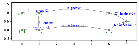
We simulate a simple toy network with a route choice option. In order to use the identical scenario in multiple simulations efficiently, we define the following function that setup a World object with the identical conditions.
[2]:
# scenario definition
def create_World():
    """
    A function that returns World object with scenario informaiton. This is faster way to reuse the same scenario, as `World.copy` or `World.load_scenario` takes some computation time.
    """
    W = uxsim.World(
        name="",
        deltan=20,
        tmax=6000,
        print_mode=0, save_mode=1, show_mode=1,
        vehicle_logging_timestep_interval=1,
        hard_deterministic_mode=False,
        random_seed=42
    )

    W.addNode("1", 0, 1)
    W.addNode("2", 1, 1)
    W.addNode("3", 5, 1)
    W.addNode("4", 0, 0)
    W.addNode("5", 1, 0)
    W.addNode("6", 5, 0)
    W.addNode("7", 6, 0.5)

    W.addLink("highway12", "1", "2", length=1000, number_of_lanes=1, merge_priority=1)
    W.addLink("highway23", "2", "3", length=3000, number_of_lanes=1, merge_priority=1, capacity_out=0.6)
    W.addLink("highway37", "3", "7", length=1000, number_of_lanes=1, merge_priority=1)
    W.addLink("onramp", "5", "2", length=1000, number_of_lanes=1, merge_priority=0.5)
    W.addLink("arterial45", "4", "5", length=1000, free_flow_speed=10, number_of_lanes=2, merge_priority=0.5)
    W.addLink("arterial56", "5", "6", length=3000, free_flow_speed=10, number_of_lanes=2, merge_priority=0.5)
    W.addLink("arterial67", "6", "7", length=1000, free_flow_speed=10, number_of_lanes=2, merge_priority=0.5)

    W.adddemand("1", "7", 0, 3000, 0.3)
    W.adddemand("4", "7", 0, 3000, 0.4*3)

    return W
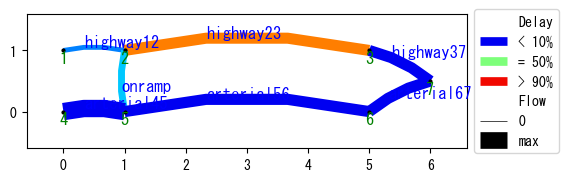
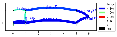
The network structure is as follows. Vehicles travel from nodes “1” and “4” at the left to node “7” at the right. The upper route is a highway, and the bottom is an arterial road. The highway has faster maximum speed but smaller traffic capacity compared with the arterial road. Vehicles from “3” can choose either highway or arterial, depending on the traffic condition.
[4]:
W = create_World()
W.show_network()
For later use, we define the following visualization function to visualize simulation results.
[5]:
def visualizaion_helper_function(W):
W.analyzer.print_simple_stats(force_print=True)
W.analyzer.network_average(legend_outside=True)
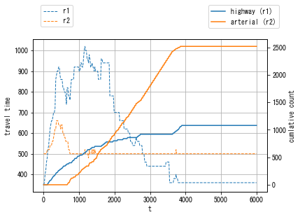
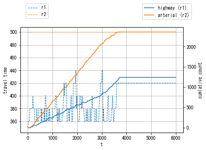
r1 = W.defRoute(["arterial45", "onramp", "highway23", "highway37"])
r2 = W.defRoute(["arterial45", "arterial56", "arterial67"])
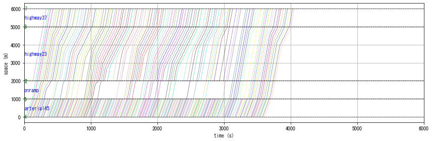
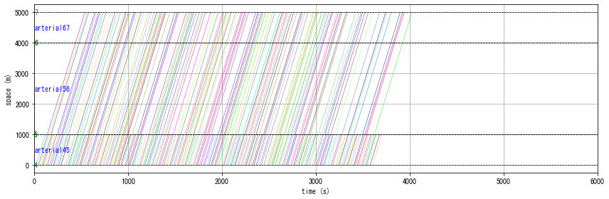
W.analyzer.time_space_diagram_traj_links(r1.links)
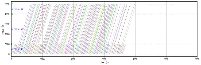
W.analyzer.time_space_diagram_traj_links(r2.links)
ttt = np.linspace(0, W.TIME, W.TSIZE)
tt1 = [r1.actual_travel_time(t) for t in ttt]
tt2 = [r2.actual_travel_time(t) for t in ttt]
fig, ax1 = subplots()
ax1.plot(ttt, tt1, "--", label="r1", lw=1)
ax1.plot(ttt, tt2, "--", label="r2", lw=1)
ax1.set_xlabel("t")
ax1.set_ylabel("travel time")
ax1.grid()
ax2 = ax1.twinx()
ax2.set_ylabel("cumlative count")
ax2.plot(ttt, W.get_link("onramp").cum_arrival, "-", label="highway (r1)")
ax2.plot(ttt, W.get_link("arterial56").cum_arrival, "-", label="arterial (r2)")
ax1.legend(loc="upper center", bbox_to_anchor=(0.1, 1.25), ncol=1)
ax2.legend(loc="upper center", bbox_to_anchor=(0.9, 1.25), ncol=1)
show()
DUO
DUO can be simulated by the default procedure of UXsim as follows.
[6]:
# DUO (default)

W_DUO = create_World()
W_DUO.exec_simulation()
W_DUO.analyzer.print_simple_stats(force_print=True)
df_DUO = W_DUO.analyzer.basic_to_pandas()

visualizaion_helper_function(W_DUO)
results:
 average speed:  9.6 m/s
 number of completed trips:      4500 / 4500
 total travel time:              4046400.0 s
 average travel time of trips:   899.2 s
 average delay of trips:         569.2 s
 delay ratio:                    0.633
 total distance traveled:        23580000.0 m
results:
 average speed:  9.6 m/s
 number of completed trips:      4500 / 4500
 total travel time:              4046400.0 s
 average travel time of trips:   899.2 s
 average delay of trips:         569.2 s
 delay ratio:                    0.633
 total distance traveled:        23580000.0 m
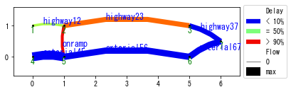
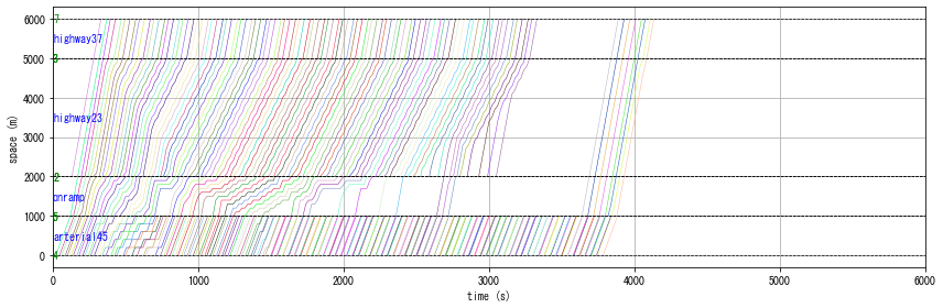
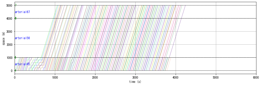
In DUO, you can see that many vehicles chose the highway route at the early stage of the simulation due to the fast maximum speed. It then caused a significant traffic jam, resulting a longer travel time. This demonstrates the myopic nature of DUO routing principle.
DUE
Approximate solution of DUE can be obtained by SolverDUE function as follows. The solution is not exact as exact DUE (in which every driver chooses the route with least travel cost) is very difficult to compute. In easy terms, the approximate DUE means that each driver chooses routes with the least expected cost when the cost is averaged for several days.
More specifically (you can skip the following explanation as it is a bit technical), this function computes a near dynamic user equilibrium state as a steady state of day-to-day dynamical routing game. On day i, vehicles choose their route based on actual travel time on day i-1 with the same departure time. If there are shorter travel time route, they will change with probability swap_prob. This process is repeated until max_iter day. It is expected that this process eventually
reach a steady state. Due to the problem complexity, it does not necessarily reach or converge to Nash equilibrium or any other stationary points. However, in the literature, it is argued that the steady state can be considered as a reasonable proxy for Nash equilibrium or dynamic equilibrium state. There are some theoretical background for it; but intuitively speaking, the steady state can be considered as a realistic state that people’s rational behavior will reach.
This method is based on the following literature:
Ishihara, M., & Iryo, T. (2015). Dynamic Traffic Assignment by Markov Chain. Journal of Japan Society of Civil Engineers, Ser. D3 (Infrastructure Planning and Management), 71(5), I_503-I_509. (in Japanese). https://doi.org/10.2208/jscejipm.71.I_503
Iryo, T., Urata, J., & Kawase, R. (2024). Traffic Flow Simulator and Travel Demand Simulators for Assessing Congestion on Roads After a Major Earthquake. In APPLICATION OF HIGH-PERFORMANCE COMPUTING TO EARTHQUAKE-RELATED PROBLEMS (pp. 413-447). https://doi.org/10.1142/9781800614635_0007
Iryo, T., Watling, D., & Hazelton, M. (2024). Estimating Markov Chain Mixing Times: Convergence Rate Towards Equilibrium of a Stochastic Process Traffic Assignment Model. Transportation Science. https://doi.org/10.1287/trsc.2024.0523
[7]:
# DUE
solver_DUE = SolverDUE(create_World)
solver_DUE.solve(max_iter=100, print_progress=False)
W_DUE = solver_DUE.W_sol
W_DUE.analyzer.print_simple_stats(force_print=True)
df_DUE = W_DUE.analyzer.basic_to_pandas()
solving DUE...
DUE summary:
 total travel time: initial 4046400.0 -> average of last 25 iters 3221200.0
 number of potential route changes: initial 1580.0 -> average of last 25 iters 1144.8
 route travel time gap: initial 57.2 -> average of last 25 iters 13.9
 computation time: 5.0 seconds
results:
 average speed:  11.3 m/s
 number of completed trips:      4500 / 4500
 total travel time:              3190400.0 s
 average travel time of trips:   709.0 s
 average delay of trips:         379.0 s
 delay ratio:                    0.535
 total distance traveled:        23840000.0 m
[8]:
visualizaion_helper_function(W_DUE)
results:
 average speed:  11.3 m/s
 number of completed trips:      4500 / 4500
 total travel time:              3190400.0 s
 average travel time of trips:   709.0 s
 average delay of trips:         379.0 s
 delay ratio:                    0.535
 total distance traveled:        23840000.0 m
[9]:
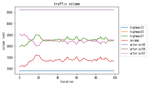
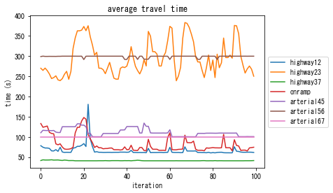
solver_DUE.plot_convergence()
solver_DUE.plot_link_stats()
solver_DUE.plot_vehicle_stats(orig="4", dest="7")
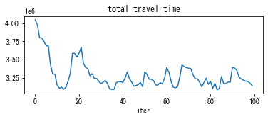
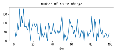
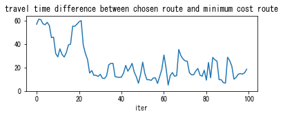
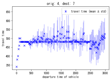
In DUE, you can see that cost is more balanced than DUO. For example, the plot “travel time difference between chosen route and minimum cost route” shows that it is reduced from 60 sec in DUO (the initial solution) to 10-20 sec in the final solution.
As a result of the travelers’ smart decision making, the total travel time of DUE is reduced to about 3 200 000 sec from 4 000 000 sec in the DUO where travelers are myopic. Note that these numbers may be different for each simulation as the algorithm is stochastic.
DSO
Now we compute DSO solution. To obtain the solution, we use a similar iterative algorithm to the previous DUE example. In this algorithm, each traveler tries to minimize their marginal travel time (i.e., private cost + externality) instead of the private cost as in DUE.
This algorithm is a loose generalization of “DSO game” of the following paper:
Satsukawa, K., Wada, K., & Watling, D. (2022). Dynamic system optimal traffic assignment with atomic users: Convergence and stability. Transportation Research Part B: Methodological, 155, 188-209.
In this paper, it is theoretically guaranteed that their DSO game algorithm converges to the global optimal DSO state. However, it may take a long time. This SolverDSO_D2D speeds up the solution process significantly, but it weakens the convergence guarantee.
[ ]:
solver_DSO = SolverDSO_D2D(create_World)
solver_DSO.solve(max_iter=50, print_progress=False)
W_DSO = solver_DSO.W_sol
W_DSO.analyzer.print_simple_stats(force_print=True)
df_DSO = W_DSO.analyzer.basic_to_pandas()
solving DSO...
DSO summary:
 total travel time: initial 4046400.0 -> minimum 2962800.0
 number of potential route changes: initial 1660.0 -> minimum 960.0
 route marginal travel time gap: initial 8825.7 -> minimum 137.5
 computation time: 2.9 seconds
results:
 average speed:  0.0 m/s
 number of completed trips:      4500 / 4500
 total travel time:              2962800.0 s
 average travel time of trips:   658.4 s
 average delay of trips:         328.4 s
 delay ratio:                    0.499
 total distance traveled:        23520000.0 m
[12]:
visualizaion_helper_function(W_DSO)
results:
 average speed:  0.0 m/s
 number of completed trips:      4500 / 4500
 total travel time:              2962800.0 s
 average travel time of trips:   658.4 s
 average delay of trips:         328.4 s
 delay ratio:                    0.499
 total distance traveled:        23520000.0 m
LoggingWarning: vehicle_logging_timestep_interval is not 1. The plot is not exactly accurate.
LoggingWarning: vehicle_logging_timestep_interval is not 1. The trajecotries are not exactly accurate.
[13]:
solver_DSO.plot_convergence()
solver_DSO.plot_link_stats()
solver_DSO.plot_vehicle_stats(orig="4", dest="7")
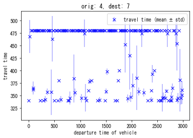
You can see that the congestion is almost eliminated. The total travel time is 3 000 000 sec in DSO. This is more efficient than DUE (with about 3 200 000 sec) or DUO (with about 4 000 000 sec).
However, some travelers are enforced to choose routes with longer travel time to improve the efficiency of the entire system.
Comparison
Comparison of 3 cases.
[15]:
df_DUO['Name'] = 'DUO'
df_DUE['Name'] = 'DUE'
df_DSO['Name'] = 'DSO'

df_combined = pd.concat([df_DUO, df_DUE, df_DSO], ignore_index=True)
cols = ['Name'] + [col for col in df_combined.columns if col != 'Name']
df_combined = df_combined[cols]
display(df_combined)
| Name | total_trips | completed_trips | total_travel_time | average_travel_time | total_delay | average_delay | |
|---|---|---|---|---|---|---|---|
| 0 | DUO | 4500 | 4500 | 4046400.0 | 899.200000 | 2561400.0 | 569.200000 |
| 1 | DUE | 4500 | 4500 | 3190400.0 | 708.977778 | 1705400.0 | 378.977778 |
| 2 | DSO | 4500 | 4500 | 2962800.0 | 658.400000 | 1477800.0 | 328.400000 |
Large-scale scenario
Now we show larger example.
[16]:
import uxsim
from uxsim import DTAsolvers
def create_World():
# simulation world
W = uxsim.World(
name="",
deltan=10,
tmax=4800,
duo_update_time=300,
print_mode=0, save_mode=0, show_mode=1,
random_seed=42,
)
# scenario
#automated network generation
#deploy nodes as an imax x jmax grid
imax = 9
jmax = 9
id_center = 4
nodes = {}
for i in range(imax):
for j in range(jmax):
nodes[i,j] = W.addNode(f"n{(i,j)}", i, j, flow_capacity=1.6)
#create links between neighborhood nodes
links = {}
for i in range(imax):
for j in range(jmax):
free_flow_speed = 10
if i != imax-1:
if j == id_center:
free_flow_speed = 20
links[i,j,i+1,j] = W.addLink(f"l{(i,j,i+1,j)}", nodes[i,j], nodes[i+1,j], length=1000, free_flow_speed=free_flow_speed)
if i != 0:
if j == id_center:
free_flow_speed = 20
links[i,j,i-1,j] = W.addLink(f"l{(i,j,i-1,j)}", nodes[i,j], nodes[i-1,j], length=1000, free_flow_speed=free_flow_speed)
if j != jmax-1:
if i == id_center:
free_flow_speed = 20
links[i,j,i,j+1] = W.addLink(f"l{(i,j,i,j+1)}", nodes[i,j], nodes[i,j+1], length=1000, free_flow_speed=free_flow_speed)
if j != 0:
if i == id_center:
free_flow_speed = 20
links[i,j,i,j-1] = W.addLink(f"l{(i,j,i,j-1)}", nodes[i,j], nodes[i,j-1], length=1000, free_flow_speed=free_flow_speed)
#generate traffic demand between the boundary nodes
demand_flow = 0.08
demand_duration = 2400
outer_ids = 3
for n1 in [(0,j) for j in range(outer_ids, jmax-outer_ids)]:
for n2 in [(imax-1,j) for j in range(outer_ids,jmax-outer_ids)]:
W.adddemand(nodes[n1], nodes[n2], 0, demand_duration, demand_flow)
for n2 in [(i,jmax-1) for i in range(outer_ids, imax-outer_ids)]:
W.adddemand(nodes[n1], nodes[n2], 0, demand_duration, demand_flow)
for n1 in [(i,0) for i in range(outer_ids, imax-outer_ids)]:
for n2 in [(i,jmax-1) for i in range(outer_ids, imax-outer_ids)]:
W.adddemand(nodes[n1], nodes[n2], 0, demand_duration, demand_flow)
for n2 in [(imax-1,j) for j in range(outer_ids,jmax-outer_ids)]:
W.adddemand(nodes[n1], nodes[n2], 0, demand_duration, demand_flow)
return W
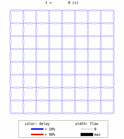
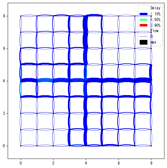
W = create_World()
W.change_print_mode(1)
W.show_network(network_font_size=0)
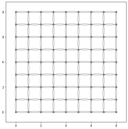
In this grid network, central links (links at x=4 and y=4) have faster free-flow speed of 20 m/s. The rest of links are with free-flow speed of 10 m/s. And the following four types of demands are generated:
bottom edge (3 nodes at (3,0), (4,0), (5,0)) to top (3 nodes at (3,8), (4,8), (5,8))
bottom edge to right
left edge to top
left to right
This is a deliberately inefficient setting that causes congestion. In a free-flowing condition, travelers tend to choose the central links. However, because traffic capacity of central links is limited, it may cause congestion although many other links are empty. To enhance system’s performance, some travelers need to be distributed to slower links to efficiently utilize the network capacity.
DUO
First, let’s compute DUO solution.
[18]:
# execute simulation
W.exec_simulation()
# visualize
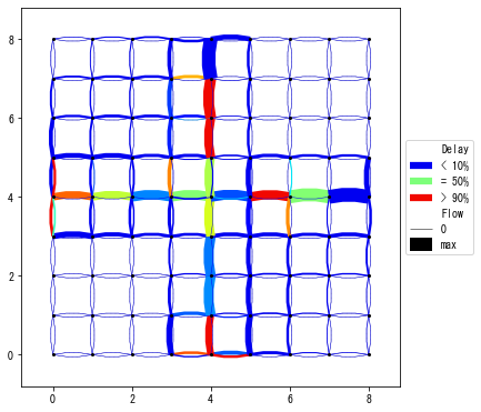
W.analyzer.print_simple_stats(force_print=True)
W.analyzer.network_average(network_font_size=0, legend=True, legend_outside=True)
W_DUO = W
df_DUO = W_DUO.analyzer.basic_to_pandas()
W_DUO.analyzer.network_anim(state_variables="flow_speed", figsize=4, animation_speed_inverse=20, timestep_skip=8, detailed=0, network_font_size=0, file_name="out/anim_DUO.gif")
uxsim.display_image_in_notebook("out/anim_DUO.gif")
    4800 s|        0 vehs|   0.0 m/s|     5.58 s
 simulation finished
results:
 average speed:  9.6 m/s
 number of completed trips:      6840 / 6840
 total travel time:              6663000.0 s
 average travel time of trips:   974.1 s
 average delay of trips:         457.5 s
 delay ratio:                    0.470
 total distance traveled:        62120000.0 m
generating animation...

The aforementioned expected behaviors are confirmed. Many travelers choose the central links first (thick width = high flow) and created congestion (red color = congestion). After that, some travelers avoided the center links. However, the overall efficiency is not good, with 0.47 delay ratio.
DUE
Now we compute DUE solution.
[19]:
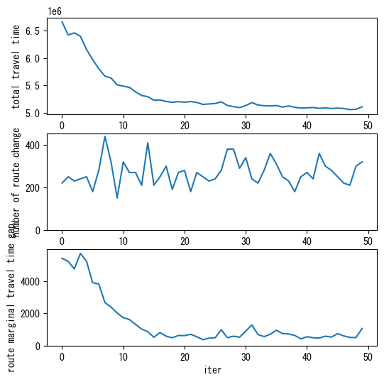
solver_DUE = DTAsolvers.SolverDUE(create_World)
solver_DUE.solve(max_iter=50, n_routes_per_od=20)

W_DUE = solver_DUE.W_sol
W_DUE.analyzer.print_simple_stats(force_print=True)
W_DUE.analyzer.network_average(network_font_size=0, legend=True)
df_DUE = W_DUE.analyzer.basic_to_pandas()

W_DUE.analyzer.network_anim(state_variables="flow_speed", figsize=4, animation_speed_inverse=20, timestep_skip=8, detailed=0, network_font_size=0, file_name="out/anim_DUE.gif")
uxsim.display_image_in_notebook("out/anim_DUE.gif")

solver_DUE.plot_convergence()
simulation setting (not finalized):
 scenario name:
 simulation duration:    4800 s
 number of vehicles:     6840 veh
 total road length:      288000 m
 time discret. width:    10 s
 platoon size:           10 veh
 number of timesteps:    480.0
 number of platoons:     684
 number of links:        288
 number of nodes:        81
 setup time:             0.01 s
number of OD pairs: 6561, number of routes: 121733
solving DUE...
 iter 0: time gap: 127.2, potential route change: 4790, route change: 230, total travel time:  6663000.0, delay ratio:  0.470
 iter 1: time gap: 129.8, potential route change: 4450, route change: 150, total travel time:  6783700.0, delay ratio:  0.479
 iter 2: time gap: 123.2, potential route change: 4500, route change: 210, total travel time:  6729100.0, delay ratio:  0.475
 iter 3: time gap: 114.3, potential route change: 4320, route change: 210, total travel time:  6662800.0, delay ratio:  0.470
 iter 4: time gap: 100.7, potential route change: 4370, route change: 240, total travel time:  6521500.0, delay ratio:  0.458
 iter 5: time gap: 102.6, potential route change: 4100, route change: 170, total travel time:  6629700.0, delay ratio:  0.467
 iter 6: time gap: 101.8, potential route change: 4230, route change: 210, total travel time:  6742800.0, delay ratio:  0.476
 iter 7: time gap: 99.2, potential route change: 4110, route change: 190, total travel time:  6594100.0, delay ratio:  0.464
 iter 8: time gap: 93.3, potential route change: 4020, route change: 180, total travel time:  6512500.0, delay ratio:  0.457
 iter 9: time gap: 99.7, potential route change: 4020, route change: 190, total travel time:  6645900.0, delay ratio:  0.468
 iter 10: time gap: 87.7, potential route change: 4090, route change: 160, total travel time:  6457500.0, delay ratio:  0.453
 iter 11: time gap: 75.6, potential route change: 4150, route change: 260, total travel time:  6215000.0, delay ratio:  0.431
 iter 12: time gap: 82.4, potential route change: 4180, route change: 200, total travel time:  6301700.0, delay ratio:  0.439
 iter 13: time gap: 76.9, potential route change: 3920, route change: 210, total travel time:  6246900.0, delay ratio:  0.434
 iter 14: time gap: 68.2, potential route change: 4030, route change: 230, total travel time:  6170400.0, delay ratio:  0.427
 iter 15: time gap: 64.8, potential route change: 4060, route change: 220, total travel time:  6053400.0, delay ratio:  0.416
 iter 16: time gap: 57.8, potential route change: 4030, route change: 220, total travel time:  5988700.0, delay ratio:  0.410
 iter 17: time gap: 60.5, potential route change: 3710, route change: 160, total travel time:  6163700.0, delay ratio:  0.427
 iter 18: time gap: 59.3, potential route change: 4160, route change: 230, total travel time:  5922700.0, delay ratio:  0.403
 iter 19: time gap: 53.2, potential route change: 3940, route change: 150, total travel time:  5941700.0, delay ratio:  0.405
 iter 20: time gap: 47.3, potential route change: 3810, route change: 220, total travel time:  5878600.0, delay ratio:  0.399
 iter 21: time gap: 55.4, potential route change: 4280, route change: 140, total travel time:  5740400.0, delay ratio:  0.384
 iter 22: time gap: 49.7, potential route change: 4180, route change: 170, total travel time:  5823800.0, delay ratio:  0.393
 iter 23: time gap: 45.2, potential route change: 4160, route change: 280, total travel time:  5738200.0, delay ratio:  0.384
 iter 24: time gap: 51.4, potential route change: 4050, route change: 220, total travel time:  5776700.0, delay ratio:  0.388
 iter 25: time gap: 44.7, potential route change: 4050, route change: 200, total travel time:  5702400.0, delay ratio:  0.380
 iter 26: time gap: 45.0, potential route change: 3820, route change: 200, total travel time:  5716400.0, delay ratio:  0.382
 iter 27: time gap: 45.3, potential route change: 3880, route change: 260, total travel time:  5729800.0, delay ratio:  0.383
 iter 28: time gap: 46.8, potential route change: 4110, route change: 140, total travel time:  5838800.0, delay ratio:  0.395
 iter 29: time gap: 43.3, potential route change: 3850, route change: 240, total travel time:  5757200.0, delay ratio:  0.386
 iter 30: time gap: 42.8, potential route change: 3730, route change: 160, total travel time:  5750400.0, delay ratio:  0.385
 iter 31: time gap: 42.5, potential route change: 3830, route change: 160, total travel time:  5704800.0, delay ratio:  0.381
 iter 32: time gap: 42.0, potential route change: 3870, route change: 170, total travel time:  5717600.0, delay ratio:  0.382
 iter 33: time gap: 40.5, potential route change: 3990, route change: 130, total travel time:  5604700.0, delay ratio:  0.369
 iter 34: time gap: 36.5, potential route change: 3620, route change: 240, total travel time:  5566100.0, delay ratio:  0.365
 iter 35: time gap: 45.5, potential route change: 4050, route change: 220, total travel time:  5610200.0, delay ratio:  0.370
 iter 36: time gap: 38.2, potential route change: 3600, route change: 190, total travel time:  5610100.0, delay ratio:  0.370
 iter 37: time gap: 38.9, potential route change: 3670, route change: 200, total travel time:  5719300.0, delay ratio:  0.382
 iter 38: time gap: 43.2, potential route change: 3780, route change: 240, total travel time:  5706300.0, delay ratio:  0.381
 iter 39: time gap: 40.6, potential route change: 3830, route change: 150, total travel time:  5685900.0, delay ratio:  0.378
 iter 40: time gap: 44.5, potential route change: 3890, route change: 190, total travel time:  5817700.0, delay ratio:  0.393
 iter 41: time gap: 44.0, potential route change: 3980, route change: 230, total travel time:  5883500.0, delay ratio:  0.399
 iter 42: time gap: 35.8, potential route change: 3890, route change: 160, total travel time:  5646000.0, delay ratio:  0.374
 iter 43: time gap: 35.6, potential route change: 3750, route change: 190, total travel time:  5649100.0, delay ratio:  0.374
 iter 44: time gap: 38.4, potential route change: 3940, route change: 240, total travel time:  5703000.0, delay ratio:  0.380
 iter 45: time gap: 37.5, potential route change: 3820, route change: 160, total travel time:  5675800.0, delay ratio:  0.377
 iter 46: time gap: 35.5, potential route change: 3850, route change: 120, total travel time:  5599600.0, delay ratio:  0.369
 iter 47: time gap: 34.9, potential route change: 3850, route change: 190, total travel time:  5506200.0, delay ratio:  0.358
 iter 48: time gap: 35.3, potential route change: 3890, route change: 200, total travel time:  5663000.0, delay ratio:  0.376
 iter 49: time gap: 33.6, potential route change: 3740, route change: 220, total travel time:  5563500.0, delay ratio:  0.365
DUE summary:
 total travel time: initial 6663000.0 -> average of last 12 iters 5674966.7
 number of potential route changes: initial 4790.0 -> average of last 12 iters 3850.8
 route travel time gap: initial 127.2 -> average of last 12 iters 38.2
 computation time: 32.4 seconds
results:
 average speed:  11.2 m/s
 number of completed trips:      6840 / 6840
 total travel time:              5563500.0 s
 average travel time of trips:   813.4 s
 average delay of trips:         296.7 s
 delay ratio:                    0.365
 total distance traveled:        59860000.0 m
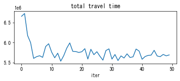
The algorithm successfully converged to a steady state, and it can be considered as a quasi-DUE state.
According to “time gap” coefficient, the DUO solution has about 140 s of time gap. This is the average time difference of route chosen by travelers and the actual minimum cost route. Since travelers in DUO are myopic, it is reasonable to have large time gap value. In the quasi-DUE state, the average time gap was reduced to about 40 s. Travelers are much smarter than DUO.
In the network animation, you can see that some travelers choose non-central links from the beginning. They anticipated that the central link would be congested and took action to avoid it in advance.
As a result, the total delay ratio was reduced to about 0.38 from 0.47 of DUO.
However, since travelers in DUE is still selfish, this is not optimal for the entire system.
DSO
Now, we compute DSO solution. Note that many local optima exist. It may be required to run the algorithm multiple times to obtain a good result.
[28]:
solver_DSO = DTAsolvers.SolverDSO_D2D(create_World)
solver_DSO.solve(max_iter=50)
W_DSO = solver_DSO.W_sol
W_DSO.analyzer.print_simple_stats(force_print=True)
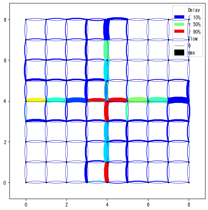
W_DSO.analyzer.network_average(network_font_size=0, legend=True)
df_DSO = W_DSO.analyzer.basic_to_pandas()
W_DSO.analyzer.network_anim(state_variables="flow_speed", figsize=4, animation_speed_inverse=20, timestep_skip=8, detailed=0, network_font_size=0, file_name="out/anim_DSO.gif")
uxsim.display_image_in_notebook("out/anim_DSO.gif")
solver_DSO.plot_convergence()
simulation setting (not finalized):
 scenario name:
 simulation duration:    4800 s
 number of vehicles:     6840 veh
 total road length:      288000 m
 time discret. width:    10 s
 platoon size:           10 veh
 number of timesteps:    480.0
 number of platoons:     684
 number of links:        288
 number of nodes:        81
 setup time:             0.01 s
number of OD pairs: 6561, number of routes: 63441
solving DSO...
 iter 0: marginal time gap: 5419.0, potential route change: 5490, route change: 220, total travel time:  6663000.0, delay ratio:  0.470
 iter 1: marginal time gap: 5231.0, potential route change: 5260, route change: 250, total travel time:  6423500.0, delay ratio:  0.450
 iter 2: marginal time gap: 4763.5, potential route change: 5350, route change: 230, total travel time:  6462300.0, delay ratio:  0.453
 iter 3: marginal time gap: 5725.8, potential route change: 5090, route change: 240, total travel time:  6401200.0, delay ratio:  0.448
 iter 4: marginal time gap: 5237.4, potential route change: 5220, route change: 250, total travel time:  6158000.0, delay ratio:  0.426
 iter 5: marginal time gap: 3904.0, potential route change: 5100, route change: 180, total travel time:  5972200.0, delay ratio:  0.408
 iter 6: marginal time gap: 3828.1, potential route change: 5120, route change: 280, total travel time:  5805300.0, delay ratio:  0.391
 iter 7: marginal time gap: 2675.1, potential route change: 5380, route change: 440, total travel time:  5669100.0, delay ratio:  0.377
 iter 8: marginal time gap: 2392.3, potential route change: 5200, route change: 320, total travel time:  5635000.0, delay ratio:  0.373
 iter 9: marginal time gap: 2026.5, potential route change: 5400, route change: 150, total travel time:  5511200.0, delay ratio:  0.359
 iter 10: marginal time gap: 1738.6, potential route change: 5560, route change: 320, total travel time:  5485100.0, delay ratio:  0.356
 iter 11: marginal time gap: 1620.2, potential route change: 5360, route change: 270, total travel time:  5463400.0, delay ratio:  0.353
 iter 12: marginal time gap: 1320.3, potential route change: 5320, route change: 270, total travel time:  5380900.0, delay ratio:  0.343
 iter 13: marginal time gap: 1029.3, potential route change: 5400, route change: 210, total travel time:  5314900.0, delay ratio:  0.335
 iter 14: marginal time gap: 861.9, potential route change: 5260, route change: 410, total travel time:  5292100.0, delay ratio:  0.332
 iter 15: marginal time gap: 518.1, potential route change: 5370, route change: 210, total travel time:  5227800.0, delay ratio:  0.324
 iter 16: marginal time gap: 808.5, potential route change: 5340, route change: 250, total travel time:  5231500.0, delay ratio:  0.324
 iter 17: marginal time gap: 584.7, potential route change: 5290, route change: 300, total travel time:  5204400.0, delay ratio:  0.321
 iter 18: marginal time gap: 486.6, potential route change: 5470, route change: 190, total travel time:  5188100.0, delay ratio:  0.319
 iter 19: marginal time gap: 629.6, potential route change: 5290, route change: 270, total travel time:  5201000.0, delay ratio:  0.321
 iter 20: marginal time gap: 619.0, potential route change: 5310, route change: 280, total travel time:  5190800.0, delay ratio:  0.319
 iter 21: marginal time gap: 700.2, potential route change: 5250, route change: 180, total travel time:  5202500.0, delay ratio:  0.321
 iter 22: marginal time gap: 549.1, potential route change: 5200, route change: 270, total travel time:  5186900.0, delay ratio:  0.319
 iter 23: marginal time gap: 367.7, potential route change: 5390, route change: 250, total travel time:  5150500.0, delay ratio:  0.314
 iter 24: marginal time gap: 462.3, potential route change: 5270, route change: 230, total travel time:  5159000.0, delay ratio:  0.315
 iter 25: marginal time gap: 485.5, potential route change: 5230, route change: 240, total travel time:  5167100.0, delay ratio:  0.316
 iter 26: marginal time gap: 981.6, potential route change: 5160, route change: 280, total travel time:  5198300.0, delay ratio:  0.320
 iter 27: marginal time gap: 493.1, potential route change: 5300, route change: 380, total travel time:  5131400.0, delay ratio:  0.311
 iter 28: marginal time gap: 583.0, potential route change: 5270, route change: 380, total travel time:  5108700.0, delay ratio:  0.308
 iter 29: marginal time gap: 524.0, potential route change: 5080, route change: 290, total travel time:  5093000.0, delay ratio:  0.306
 iter 30: marginal time gap: 904.7, potential route change: 5190, route change: 340, total travel time:  5129500.0, delay ratio:  0.311
 iter 31: marginal time gap: 1282.6, potential route change: 5040, route change: 240, total travel time:  5184500.0, delay ratio:  0.318
 iter 32: marginal time gap: 687.0, potential route change: 5170, route change: 220, total travel time:  5138900.0, delay ratio:  0.312
 iter 33: marginal time gap: 558.3, potential route change: 5240, route change: 280, total travel time:  5126700.0, delay ratio:  0.311
 iter 34: marginal time gap: 700.1, potential route change: 5080, route change: 360, total travel time:  5122600.0, delay ratio:  0.310
 iter 35: marginal time gap: 956.5, potential route change: 5220, route change: 310, total travel time:  5130600.0, delay ratio:  0.311
 iter 36: marginal time gap: 747.5, potential route change: 5200, route change: 250, total travel time:  5101900.0, delay ratio:  0.307
 iter 37: marginal time gap: 722.5, potential route change: 5220, route change: 230, total travel time:  5122100.0, delay ratio:  0.310
 iter 38: marginal time gap: 631.3, potential route change: 5210, route change: 180, total travel time:  5098000.0, delay ratio:  0.307
 iter 39: marginal time gap: 418.5, potential route change: 5170, route change: 250, total travel time:  5083000.0, delay ratio:  0.305
 iter 40: marginal time gap: 551.7, potential route change: 5310, route change: 270, total travel time:  5087600.0, delay ratio:  0.305
 iter 41: marginal time gap: 485.2, potential route change: 5000, route change: 240, total travel time:  5093600.0, delay ratio:  0.306
 iter 42: marginal time gap: 468.1, potential route change: 5240, route change: 360, total travel time:  5078400.0, delay ratio:  0.304
 iter 43: marginal time gap: 582.0, potential route change: 5180, route change: 300, total travel time:  5086500.0, delay ratio:  0.305
 iter 44: marginal time gap: 527.3, potential route change: 5180, route change: 280, total travel time:  5074400.0, delay ratio:  0.304
 iter 45: marginal time gap: 746.8, potential route change: 5000, route change: 250, total travel time:  5083000.0, delay ratio:  0.305
 iter 46: marginal time gap: 600.5, potential route change: 5170, route change: 220, total travel time:  5074200.0, delay ratio:  0.304
 iter 47: marginal time gap: 508.6, potential route change: 5230, route change: 210, total travel time:  5054400.0, delay ratio:  0.301
 iter 48: marginal time gap: 498.3, potential route change: 5170, route change: 300, total travel time:  5060900.0, delay ratio:  0.302
 iter 49: marginal time gap: 1060.3, potential route change: 4890, route change: 320, total travel time:  5106100.0, delay ratio:  0.308
DSO summary:
 total travel time: initial 6663000.0 -> minimum 5054400.0
 number of potential route changes: initial 5490.0 -> minimum 4890.0
 route marginal travel time gap: initial 5419.0 -> minimum 367.7
 computation time: 42.2 seconds
results:
 average speed:  0.0 m/s
 number of completed trips:      6840 / 6840
 total travel time:              5054400.0 s
 average travel time of trips:   738.9 s
 average delay of trips:         222.3 s
 delay ratio:                    0.301
 total distance traveled:        61180000.0 m

Now the traffic situation is much better, with 0.31 delay ratio. According to the network animation, traffic was distributed to many routes. Most of traffic congestion observed in DUO/DUE solutions were eliminated.
Below is the summary of the 3 scenarios.
[29]:
df_DUO['Name'] = 'DUO'
df_DUE['Name'] = 'DUE'
df_DSO['Name'] = 'DSO'

df_combined = pd.concat([df_DUO, df_DUE, df_DSO], ignore_index=True)
cols = ['Name'] + [col for col in df_combined.columns if col != 'Name']
df_combined = df_combined[cols]
display(df_combined)
| Name | total_trips | completed_trips | total_travel_time | average_travel_time | total_delay | average_delay | |
|---|---|---|---|---|---|---|---|
| 0 | DUO | 6840 | 6840 | 6663000.0 | 974.122807 | 3129000.0 | 457.456140 |
| 1 | DUE | 6840 | 6840 | 5563500.0 | 813.377193 | 2029500.0 | 296.710526 |
| 2 | DSO | 6840 | 6840 | 5054400.0 | 738.947368 | 1520400.0 | 222.280702 |
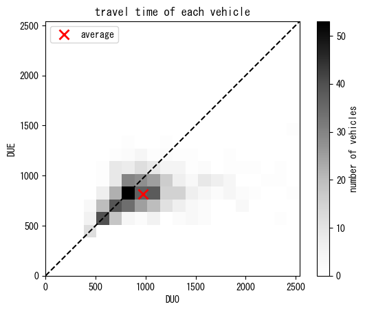
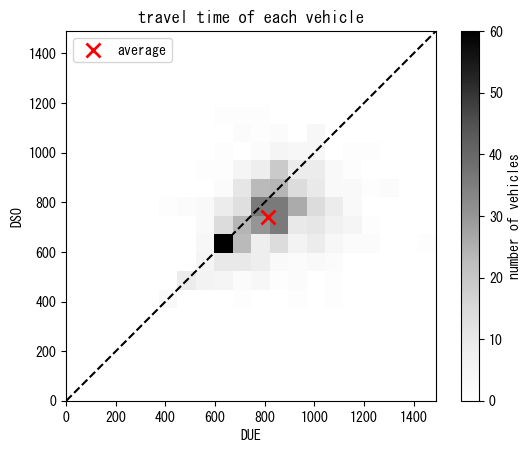
Below is some vehicle-level analysis. You can see that, on average, travel time in DUE is shorter than that of DUO, and that in DSO is shorter than that of DUE. This indicates overall efficiency of respective route choice principles. However, from the perspective of each individual vehicles, some of them experience longer travel time in DSO than DUE. This can be a potential fairness issue.
[43]:
travel_time_per_vehicle_duo = [veh.travel_time for veh in W_DUO.VEHICLES.values()]
travel_time_per_vehicle_due = [veh.travel_time for veh in W_DUE.VEHICLES.values()]
travel_time_per_vehicle_dso = [veh.travel_time for veh in W_DSO.VEHICLES.values()]

figure()
subplot(111, aspect="equal")
title("travel time of each vehicle")
max_val = max(max(travel_time_per_vehicle_duo), max(travel_time_per_vehicle_due))
plot([0, max_val], [0, max_val], "k--")
hist2d(travel_time_per_vehicle_duo, travel_time_per_vehicle_due, range=[[0, max_val], [0, max_val]], bins=20, cmap="Greys")
plot(average(travel_time_per_vehicle_duo), average(travel_time_per_vehicle_due), "rx", ms=10, mew=2, label="average")
colorbar().set_label("number of vehicles")
xlabel("DUO")
ylabel("DUE")
legend()
show()

figure()
subplot(111, aspect="equal")
title("travel time of each vehicle")
max_val = max(max(travel_time_per_vehicle_due), max(travel_time_per_vehicle_dso))
plot([0, max_val], [0, max_val], "k--")
hist2d(travel_time_per_vehicle_due, travel_time_per_vehicle_dso, range=[[0, max_val], [0, max_val]], bins=20, cmap="Greys")
plot(average(travel_time_per_vehicle_due), average(travel_time_per_vehicle_dso), "rx", ms=10, mew=2, label="average")
colorbar().set_label("number of vehicles")
xlabel("DUE")
ylabel("DSO")
legend()
show()