Step-by-step Tutorial

This tutorial demonstrates how to use the UXsim package to simulate traffic scenarios and analyze the results using Python in a Jupyter Notebook environment.

%matplotlib inline

Simple Scenario Example

First, import the required module.

from uxsim import *

Scenario Definition

First, we will define the main simulation world W. The simulation scenario is defined by creating an object of the World class, which represents the main simulation environment. The constructor takes several parameters. The unit of time is s (seconds) and the unit of length is m (meters).

• name: A string specifying the name of the scenario. This is used as the folder name for saving results. It can be left blank.

• deltan: An integer specifying the simulation aggregation unit Δn, which defines how many vehicles are grouped together (i.e., platoon size) for computation.

• tmax: An integer specifying the total simulation time in seconds.

• print_mode: An integer (0 or 1) determining whether to print information during the simulation. Usually set to 1, but recommended 0 when running multiple simulations automatically.

• save_mode: An integer (0 or 1) determining if visualization results are saved.

• show_mode: An integer (0 or 1) determining if visualization results are displayed. It’s good to set show_mode=1 in Jupyter Notebook, otherwise recommended 0.

• random_seed: A random seed for reproducible experiments. Set to None for non-deterministic behavior.

W = World(
    name="simple_demo",    # Scenario name. Can be blank. Used as the folder name for saving results.
    deltan=5,   # Simulation aggregation unit Δn. Defines how many vehicles are grouped together (i.e., platoon size) for computation. Computation cost is generally inversely proportional to deltan^2.
    tmax=1200,  # Total simulation time (s)
    print_mode=1, save_mode=1, show_mode=1,    # Various options. print_mode determines whether to print information. Usually set to 1, but recommended 0 when running multiple simulations automatically. save_mode determines if visualization results are saved. show_mode determines if visualization results are displayed. It's good to set show_mode=1 on Jupyter Notebook, otherwise recommended 0.
    random_seed=0    # Set the random seed. Specify if you want repeatable experiments. If not, set to None.
)

Next, the nodes and links of the network are defined using the addNode (to add Node object) and addLink (to add Link object) methods of the World object. The addNode method requires the following parameters:

• name: A string specifying the name of the node.

• x: A float specifying the x-coordinate of the node for visualization purposes.

• y: A float specifying the y-coordinate of the node for visualization purposes.

The addLink method requires the following parameters (some of them are optional though):

• name: A string specifying the name of the link.

• start_node: A string specifying the name of the start node. You can also specify Node object instead.

• end_node: A string specifying the name of the end node. You can also specify Node object instead.

• length: A float specifying the length of the link.

• free_flow_speed: A float specifying the free flow speed of the link.

• number_of_lanes: An integer specifying the number of lanes of the link.

• merge_priority: A float specifying the merge priority of the link during merging.

W.addNode("orig1", 0, 0) #Create a node. Parameters: node name, visualization x-coordinate, visualization y-coordinate
W.addNode("orig2", 0, 2)
W.addNode("merge", 1, 1)
W.addNode("dest", 2, 1)

W.addLink("link1", "orig1", "merge", length=1000, free_flow_speed=20, number_of_lanes=1, merge_priority=0.5) # Create a link. Parameters: link name, start node, end node, length, free_flow_speed, number of lanes, merge_priority during merging
W.addLink("link2", "orig2", "merge", length=1000, free_flow_speed=20, number_of_lanes=1, merge_priority=2)
W.addLink("link3", "merge", "dest", length=1000, free_flow_speed=20, number_of_lanes=1)

<Link link3>

Finally, the traffic demand between origin-destination (OD) pairs is specified using the adddemand method, which add appropriate number of Vehicle objects. It requires the following parameters:

• orig: A string specifying the name of the origin node. You can also specify Node object instead.

• dest: A string specifying the name of the destination node. You can also specify Node object instead.

• t_start: A float specifying the start time of the demand in seconds.

• t_end: A float specifying the end time of the demand in seconds.

• flow: A float specifying the demand flow rate in vehicles per second.

W.adddemand("orig1", "dest", 0, 1000, 0.4) # Create OD traffic demand. Parameters: origin node, destination node, start time, end time, demand flow rate
W.adddemand("orig2", "dest", 500, 1000, 0.6)

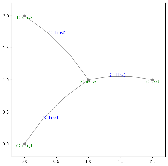
You can check the network shape by using W.show_network() (Note that the plot uses left-handed traffic rule). This scenario is a simple Y-shaped network. It may cause traffic congestion due to merging.

W.show_network()

Simulation Execution

Once the scenario is defined, the simulation can be executed by calling the exec_simulation method of the World object. It first show the summary of the simulation setting, the following information is printed during the simulation to see the progress:

• Current simulation time

• Number of vehicles in the network

• Average speed of vehicles

• Computation time taken for the simulation steps so far

W.exec_simulation()

simulation setting:
 scenario name: simple_demo
 simulation duration:    1200 s
 number of vehicles:     700 veh
 total road length:      3000 m
 time discret. width:    5 s
 platoon size:           5 veh
 number of timesteps:    240
 number of platoons:     140
 number of links:        3
 number of nodes:        4
 setup time:             5.82 s
simulating...
      time| # of vehicles| ave speed| computation time
       0 s|        0 vehs|   0.0 m/s|     0.00 s
     600 s|      100 vehs|  17.5 m/s|     0.05 s
    1195 s|       25 vehs|  20.0 m/s|     0.09 s
 simulation finished

1

The simulation can also be run in steps by specifying the duration_t parameter of exec_simulation. This allows intervening in the simulation at intermediate points. This is for advantage usage. For example:

while W.check_simulation_ongoing():
    W.exec_simulation(duration_t=100)
    your_intervention_method()

Results Analysis

The Analyzer class accessible as W.analyzer is responsible for analyzing the results.

A summary of the results can be printed below. Delay ratio is the ratio of delay time to total trip time, with a value close to zero indicating smooth traffic (when the shortest route can be traveled without congestion) and a larger value indicating congestion (when the shortest route is bypassed or congested).

W.analyzer.print_simple_stats()

results:
 average speed:  13.8 m/s
 number of completed trips:      675 / 700
 average travel time of trips:   142.7 s
 average delay of trips:         42.7 s
 delay ratio:                    0.299

Simulation results can be output as pandas.DataFrame objects by using the following functions. Note that the value -1 basically means undefined (e.g., headway when there is no vehicle in front).

#overall
df = W.analyzer.basic_to_pandas()
display(df)

#OD-specific traffic situation
df = W.analyzer.od_to_pandas()
display(df)

#MFD
df = W.analyzer.mfd_to_pandas()
display(df)

#link-level
df = W.analyzer.link_to_pandas()
display(df)

#within link
df = W.analyzer.link_traffic_state_to_pandas()
display(df)

#vehicle-level
df = W.analyzer.vehicles_to_pandas()
display(df)

	total_trips	completed_trips	total_travel_time	average_travel_time	total_delay	average_delay
0	700	675	96325.0	142.703704	28825.0	42.703704

	orig	dest	total_trips	completed_trips	free_travel_time	average_travel_time	stddiv_travel_time
0	orig1	dest	400	375	100.0	167.666667	89.388043
1	orig2	dest	300	300	100.0	111.500000	5.188127

	t	network_k	network_q
0	0	0.006944	0.138889

	link	start_node	end_node	traffic_volume	vehicles_remain	free_travel_time	average_travel_time	stddiv_travel_time
0	link1	orig1	merge	400	0	50.0	128.125000	82.211776
1	link2	orig2	merge	300	0	50.0	55.208333	5.548868
2	link3	merge	dest	675	25	50.0	52.166667	2.477678

	link	t	x	delta_t	delta_x	q	k	v
0	link1	0	0.0	120	100.0	0.375000	0.018750	20.0
1	link1	0	100.0	120	100.0	0.333333	0.016667	20.0
2	link1	0	200.0	120	100.0	0.333333	0.016667	20.0
3	link1	0	300.0	120	100.0	0.333333	0.016667	20.0
4	link1	0	400.0	120	100.0	0.291667	0.014583	20.0
...	...	...	...	...	...	...	...	...
295	link3	1080	500.0	120	100.0	0.770833	0.038542	20.0
296	link3	1080	600.0	120	100.0	0.770833	0.038542	20.0
297	link3	1080	700.0	120	100.0	0.760417	0.038021	20.0
298	link3	1080	800.0	120	100.0	0.760417	0.038021	20.0
299	link3	1080	900.0	120	100.0	0.791667	0.039583	20.0

300 rows × 8 columns

	name	dn	orig	dest	t	link	x	s	v
0	0	5	orig1	dest	15	link1	0.0	-1.0	20.0
1	0	5	orig1	dest	20	link1	100.0	-1.0	20.0
2	0	5	orig1	dest	25	link1	200.0	-1.0	20.0
3	0	5	orig1	dest	30	link1	300.0	-1.0	20.0
4	0	5	orig1	dest	35	link1	400.0	-1.0	20.0
...	...	...	...	...	...	...	...	...	...
4207	139	5	orig2	dest	1090	link3	600.0	225.0	20.0
4208	139	5	orig2	dest	1095	link3	700.0	225.0	20.0
4209	139	5	orig2	dest	1100	link3	800.0	-1.0	20.0
4210	139	5	orig2	dest	1105	link3	900.0	-1.0	20.0
4211	139	5	orig2	dest	1105	trip_end	-1.0	-1.0	-1.0

4212 rows × 9 columns

You can also save these results to CSV using

W.analyzer.output_data()

Visualization of Results

Several visualization methods are provided to confirm the simulation results.

Link-level

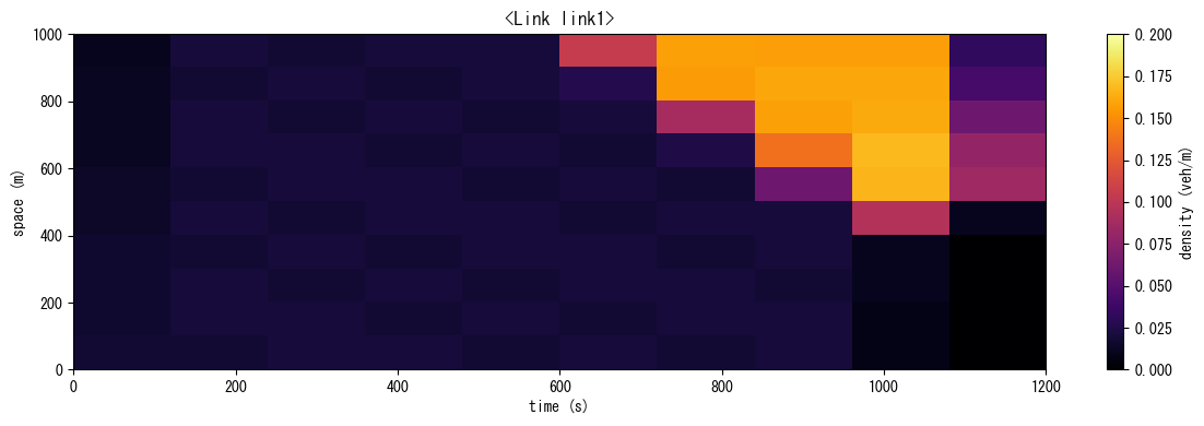
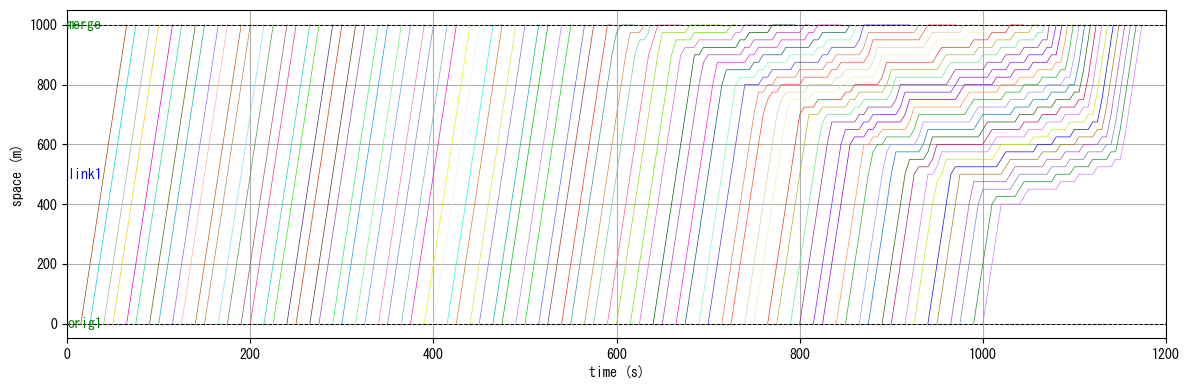
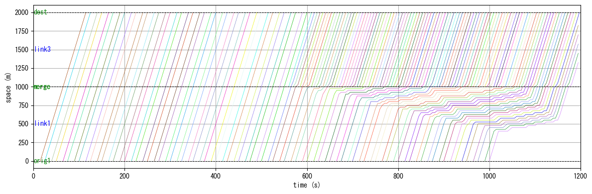
Time-space diagrams (density and trajectories) of a link can be plotted as follows. Ones for consecutive links can also be plotted.

W.analyzer.time_space_diagram_density("link1")
W.analyzer.time_space_diagram_traj("link1")

W.analyzer.time_space_diagram_traj_links([["link1", "link3"]])

 drawing traffic states...

 drawing trajectories...

 drawing trajectories...

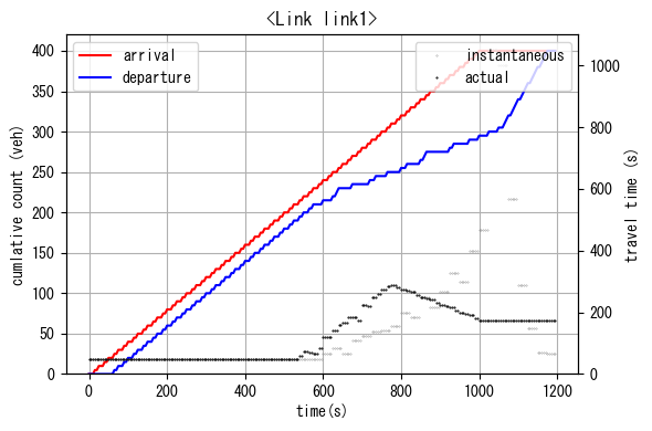
Cumulative curves (with actual/instantaneous travel times) can be plotted by using

W.analyzer.cumulative_curves(["link1"])

Network/Area-level

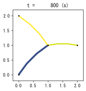
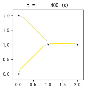
Network traffic states can be visualized by number of ways:

• W.analyzer.network(t, detailed=0): Snapshots of link-average traffic states

• W.analyzer.network(t, detailed=1): Snapshots of segment-level traffic states

• W.analyzer.network_anim: Dynamic animation of network traffic states

• W.analyzer.network_fancy: Dynamic animation of vehicle trajectories in network

By default, you can visualize the traffic situation per link, the traffic situation per segment within a link (not very clear depending on the network geometry), and the movement trajectory of some vehicles. The thicker the width of the link, the greater the number and density of vehicles, and the darker the color, the lower the speed. Note that the animation generation speed for large scenarios could take some time.

Note also that this example uses left-handed traffic rule (e.g., Japan, UK). If you want to use right-handed one, you need to specify option left_handed=0.

for t in list(range(0,W.TMAX,int(W.TMAX/3))):
    W.analyzer.network(t, detailed=0, network_font_size=0, figsize=(3,3))
for t in list(range(0,W.TMAX,int(W.TMAX/3))):
    W.analyzer.network(t, detailed=1, network_font_size=0, figsize=(3,3))

W.analyzer.network_anim(animation_speed_inverse=15, timestep_skip=30, detailed=0, figsize=(6,6), network_font_size=0)
from IPython.display import display, Image
with open("outsimple_demo/anim_network0.gif", "rb") as f:
    display(Image(data=f.read(), format='png'))

W.analyzer.network_anim(detailed=1, figsize=(6,6), network_font_size=0)

with open("outsimple_demo/anim_network1.gif", "rb") as f:
    display(Image(data=f.read(), format='png'))

W.analyzer.network_fancy(animation_speed_inverse=15, sample_ratio=0.3, interval=3, trace_length=3, network_font_size=0)

with open("outsimple_demo/anim_network_fancy.gif", "rb") as f:
    display(Image(data=f.read(), format='png'))

 generating animation...

 generating animation...

 generating animation...

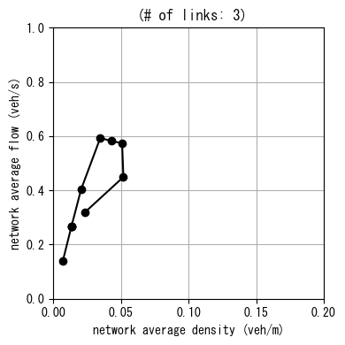
MFD (Macroscopic fundamental diagram), which summarizes the whole network states, can also be plotted by using

W.analyzer.macroscopic_fundamental_diagram()

GUI for interactive exploration

You can also launch GUI viewer for interactive exploration. It can play and pause network traffic animation, show time-space diagrams of selected links, track specific vehicles, see some statistics, and export these results to CSVs.

from uxsim.ResultGUIViewer import ResultGUIViewer
ResultGUIViewer.launch_World_viewer(W)

Sioux Falls Network

The tutorial concludes with a larger example applying the package to simulate the well-known Sioux Falls network, often used as a benchmark in transportation research.

The most frequently used functions would be those of World (to define simulation scenarios) and Analyzer (to analyze simulation results). For the details, please refer to the technical reference: https://toruseo.jp/UXsim/docs/tech_ref.html.

# Simulation main
W = World(
    name="simple_demo",
    deltan=5,
    tmax=7200,
    print_mode=1, save_mode=1, show_mode=0,
    random_seed=0
)

# Scenario definition
W.load_scenario("dat/sfnetwork.uxsim_scenario")

# Simulation execution
W.exec_simulation()

# Results analysis
W.analyzer.print_simple_stats()

loading scenario from 'dat/sfnetwork.uxsim_scenario'
 DATA SOURCE AND LICENCE : Sioux Falls network. This is based on https://github.com/bstabler/TransportationNetworks/tree/master/SiouxFalls by Transportation Networks for Research Core Team. Users need to follow their licence. Especially, this data is for academic research purposes only, and users must indicate the source of any dataset they are using in any publication that relies on any of the datasets provided in this web site.
 Number of loaded nodes: 24
 Number of loaded links: 76
 Number of loaded `adddemand`s: 1056
simulation setting:
 scenario name: simple_demo
 simulation duration:    7200 s
 number of vehicles:     34690 veh
 total road length:      314000.0 m
 time discret. width:    5 s
 platoon size:           5 veh
 number of timesteps:    1440
 number of platoons:     6938
 number of links:        76
 number of nodes:        24
 setup time:             0.58 s
simulating...
      time| # of vehicles| ave speed| computation time
       0 s|        0 vehs|   0.0 m/s|     0.00 s
     600 s|     2550 vehs|   7.2 m/s|     1.80 s
    1200 s|     5815 vehs|   6.9 m/s|     4.01 s
    1800 s|     8700 vehs|   6.5 m/s|     6.47 s
    2400 s|    10335 vehs|   5.8 m/s|     9.04 s
    3000 s|    10955 vehs|   5.3 m/s|    11.63 s
    3600 s|    13390 vehs|   4.9 m/s|    14.69 s
    4200 s|    14265 vehs|   4.5 m/s|    17.07 s
    4800 s|    15175 vehs|   4.4 m/s|    19.70 s
    5400 s|    11190 vehs|   5.4 m/s|    22.08 s
    6000 s|     6745 vehs|   6.0 m/s|    23.30 s
    6600 s|     3460 vehs|   6.1 m/s|    24.03 s
    7195 s|     1525 vehs|   6.2 m/s|    24.39 s
 simulation finished
results:
 average speed:  5.4 m/s
 number of completed trips:      33165 / 34690
 average travel time of trips:   1751.1 s
 average delay of trips:         383.5 s
 delay ratio:                    0.219

from uxsim.ResultGUIViewer import ResultGUIViewer
ResultGUIViewer.launch_World_viewer(W)

W.analyzer.network_anim(animation_speed_inverse=15, timestep_skip=8, detailed=0, network_font_size=0)
with open("outsimple_demo/anim_network0.gif", "rb") as f:
    display(Image(data=f.read(), format='png'))

 generating animation...