Simulation Mechanism: Summary

In this page, we briefly explain the models and logics behind UXsim. If you want to know more details, please refer to arXiv preprint on UXsim, the code, the original articles, or Japanese textbook on traffic simulation.

Models

UXsim computes network traffic flow dynamics by combining following models:

• The mesoscopic version of Newell’s simplified car-following model (aka. X-model) for vehicle behavior in link.

• The mesoscopic version of the incremental node model for inter-link transfer at nodes. It includes bottlenecks and traffic signals.

• A modified dynamic user optimum (aka. reactive assignment) for route choice of travelers. Basically, travelers choose the minimum travel time route considering the latest traffic situation.

Key Inputs

UXsim’s key inputs (i.e., simulation scenario parameters) are as follows:

• Reaction time of vehicles (reaction_time argument of World). This value determines the simulation time step width. This is a global parameter.

• Platoon size for mesoscopic simulation (deltan of World). This value determines the simulation time step width. This is a global parameter.

• Route choice model parameters: shortest path update interval (duo_update_time of World) and weight value (duo_update_weight of World).

• Lists of nodes and links. They define the network structure.

• Parameters of each link. For example, length, free flow speed (free_flow_speed), number of lanes (number_of_lanes), jam density (jam_density), merging priority parameter (merge_priority), and traffic signal setting (signal_group).

• Parameters of each node. For example, position (x and y) and traffic signal setting (signal).

• Demand. For example, origin, destination, and departure time of each vehicle are specified.

Simulation Framework

In this section, the logical flow of the simulation is explained.

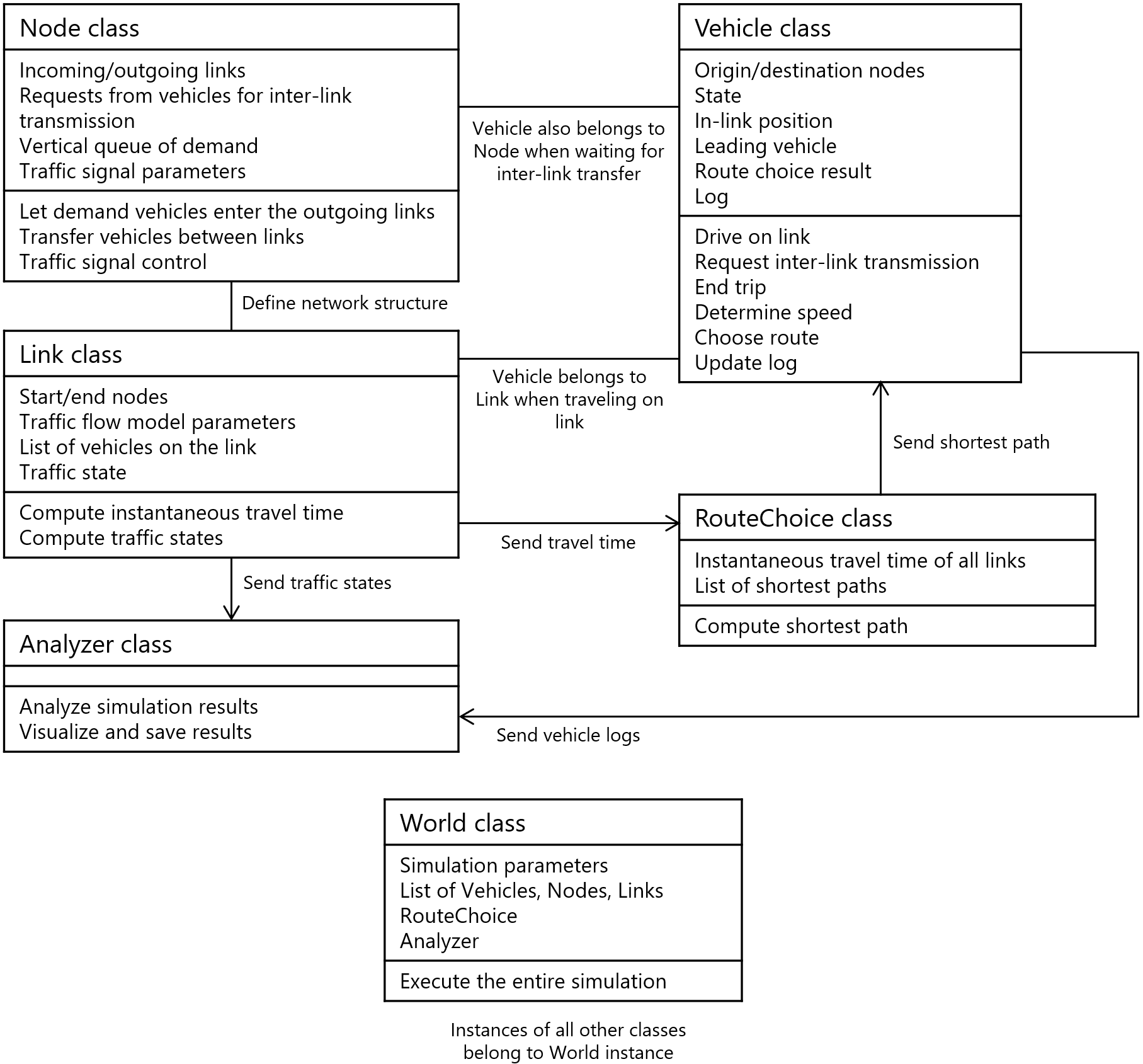
Program Structure

Class diagram of UXsim: the relationship between classes and their key properties.

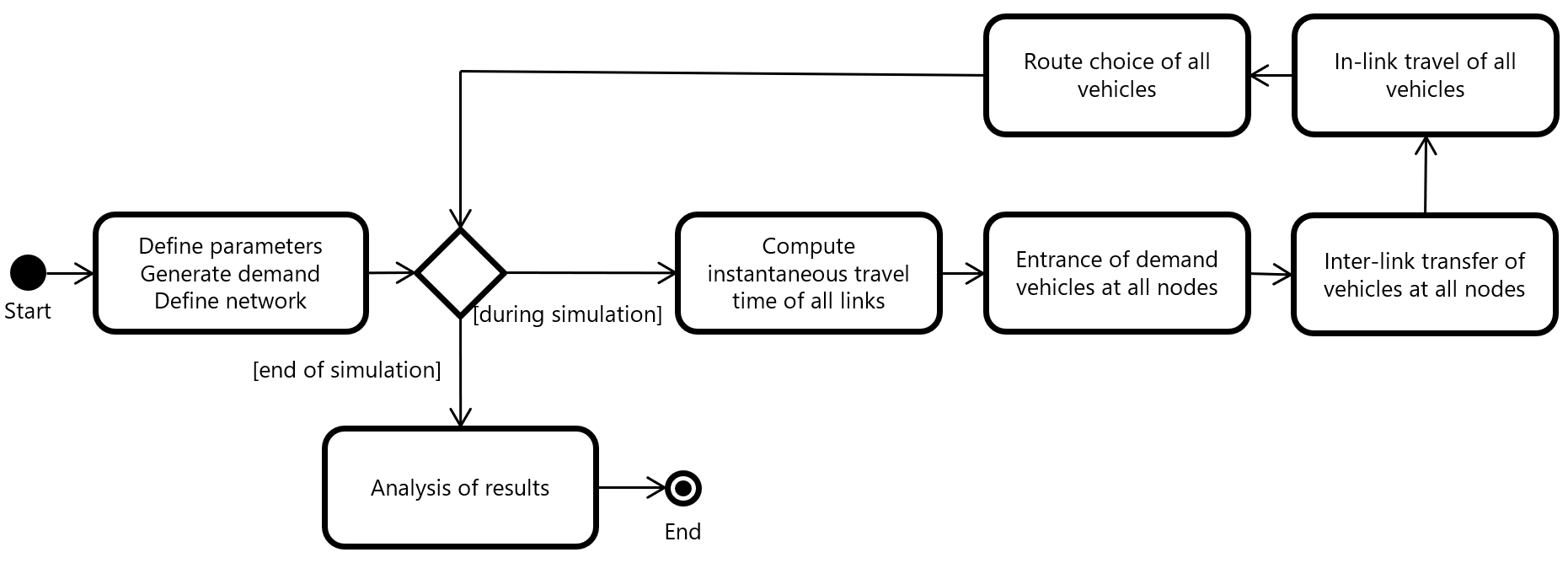
Computation Procedure

Activity diagram of UXsim: the overall computation procedure of UXsim.

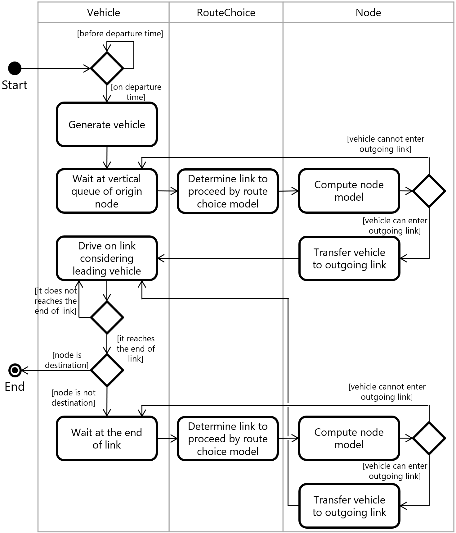
Activity diagram of a specific vehicle in UXsim: the computation procedure for each vehicle.

Traffic Flow Model

In this section, the model used for vehicle driving behavior on a link is explained. This section may be too technical and can be skipped.

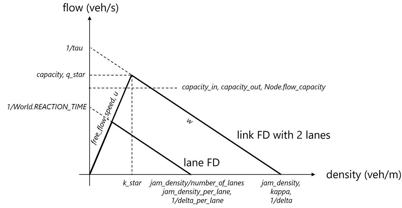
Model Parameters

The following parameters are used in UXsim, defined through Link, World, and Node (*: input, **: alternative input). If you are not familiar with the traffic flow theory, it is recommended that you adjust only free_flow_speed and number_of_lanes for the traffic flow model parameters, leaving the other parameters at their default values.

• * free_flow_speed (m/s)

• * jam_density (veh/m/LINK)

• ** jam_density_per_lane (veh/m/lane)

• * lanes, number_of_lane (lane)

• tau: y-intercept of link FD (s/veh*LINK)

• REACTION_TIME (s/veh*lane)

• w (m/s)

• capacity (veh/s/LINK)

• capacity_per_lane (veh/s/lane)

• delta: minimum spacing (m/veh*LINK)

• delta_per_lane: minimum spacing in lane (m/veh*lane)

• q_star: capacity (veh/s/LINK)

• k_star: critical density (veh/s/LINK)

• * capacity_in, capacity_out: bottleneck capacity at beginning/end of link (veh/s/LINK)

• * Node.flow_capacity: node flow capacity (veh/s/LINK-LIKE)

Newell’s Simplified Car-Following Model

The Newell’s simplified car-following model is a simple yet essential traffic flow model that describes vehicle movement based on the principle that drivers maintain a safe following distance from the vehicle ahead. It’s known for its simplicity and computational efficiency.

The Newell model can be considered as a simple approximation of standard car-following models such as Nagel-Schreckenberg (cellar automata), Gipps (used by a commercial software), and Krauss (used by SUMO) models. This suggests that the Newell model captures some of the universal essence of car-following models.

Key Variables

• Position: \(x_n^t\) represents the position of vehicle \(n\) at time \(t\)

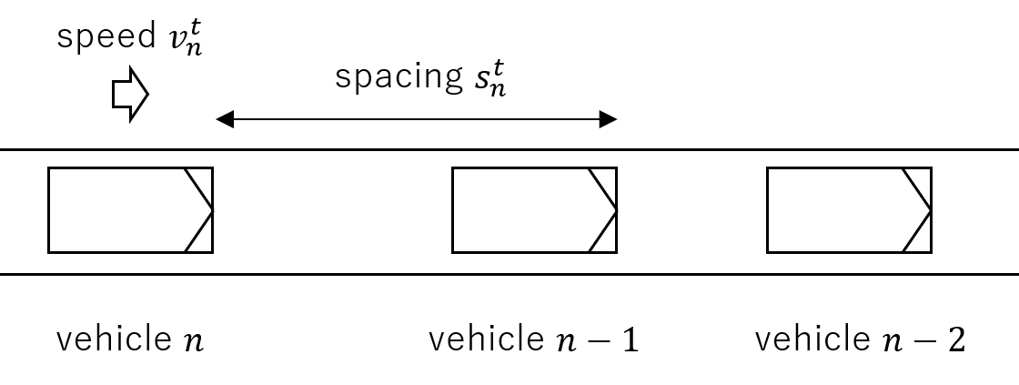
• Speed: \(v_n^t\) represents the speed of vehicle \(n\) at time \(t\)

  • Mathematically: \(v_n^t = \frac{x_n^t - x_n^{t-1}}{\tau}\)

• Spacing: \(s_n^t\) represents the spacing between vehicle \(n\) and the leading vehicle \(n-1\) at time \(t\)

  • Mathematically: \(s_n^t = x_{n-1}^t - x_n^t\)

• Reaction time: \(\tau\) is the driver’s reaction time

• Minimum spacing: \(\delta\) is the minimum distance between vehicles when stationary

• Free-flow speed: \(u\) is the maximum speed a vehicle can travel in uncongested conditions

Basic Mechanism

The Newell model determines a vehicle’s position based on the position of the vehicle ahead, with a time delay to account for reaction time. The model assumes that:

1. Each driver attempts to maintain a safe following distance

2. The vehicle will travel at free-flow speed if there is sufficient spacing

3. Otherwise, the vehicle adjusts its speed to maintain safety

The core equation of the Newell model is:

\[x_n^{t+\tau} = \min\{x_n^t + u\tau, x_{n-1}^t - \delta\}\]

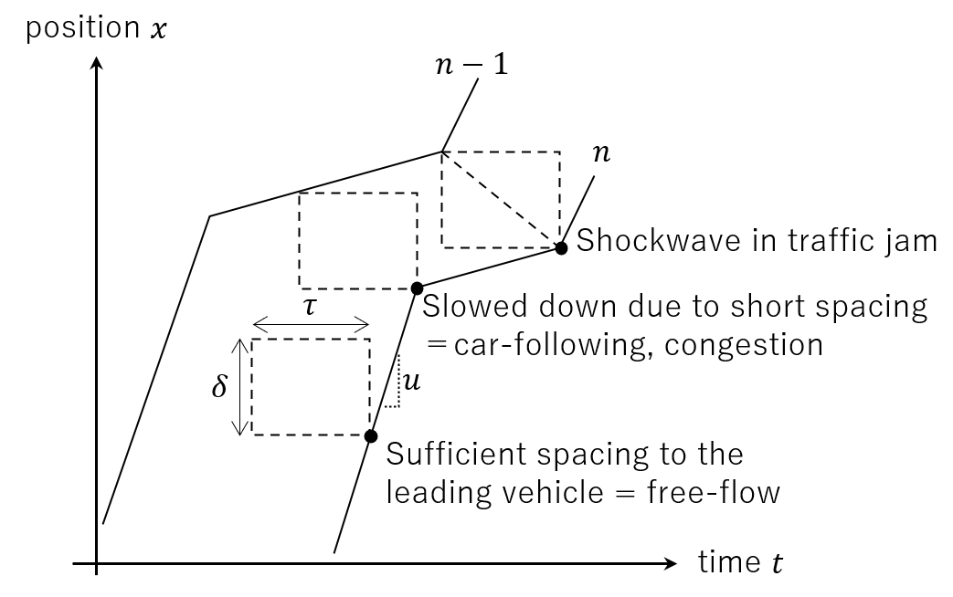
This means that the position of vehicle \(n\) at time \(t+\tau\) is determined by taking the minimum of:

• The position it would reach traveling at free-flow speed (\(x_n^t + u\tau\))

• The position of the leading vehicle minus the minimum spacing (\(x_{n-1}^t - \delta\)), meaning that vehicle \(n\) is following its leading vehicle. In this case, vehicle \(n\) may be slowed down due to the leading vehicle, and traffic may be congested

In a time-space diagram, the behavior of this model can be depicted as follows.

Mesoscopic Newell Model

By considering \(\Delta n\) consecutive vehicles as a single entity like a platoon or packet, the Newell model can be computed very efficiently. We call it the mesoscopic version of Newell model

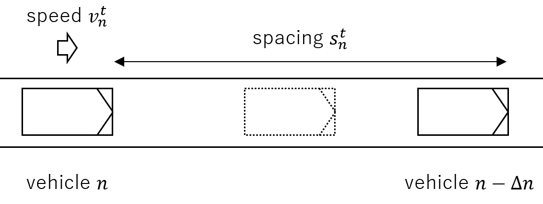
The model formula is:

\[x_n^{t+\tau\Delta n} = \min\{x_n^t + u\tau, x_{n-\Delta n}^t - \delta\Delta n\}\]

The advantage of this model:

• Exactly accurate for link-level traffic: No numerical error compared with the original model. There is a theory reason.

• Computationally efficient: Now we only compute 1 vehicle per \(\Delta n\) vehicles. Furthermore, timestep width is \(\tau\Delta n\). Thus, the computational cost is proportional to \(1/\Delta n ^2\).

The limitation:

• Aggregation error at network-level traffic: All vehicles in single platoon must have the same OD pair and travel the same route consecutively. This can be a source of errors at node merging/diverging and route choice behaviors.