[3]:
%matplotlib inline
Huge-scale simulation using Chicago-Sketch dataset
In this example, we demonstrate how UXsim can be used for huge-scale simulation in metropolitan area. We use Chicago-Sketch dataset provided by Transportation Networks for Research. The scenario data for UXsim is derived from the original TNTP dataset and provided as chicago_sketch.uxsim_scenario at UXsim repo. The code generated UXsim scenario file is attached to the end of this notebook.
The dataset contains an abstract road network of Chicago metropolitan area with 546 nodes and 2176 links. The traffic demand is almost 1 million vehicles for 1 hour in the peak period. Note that the data is modified from the original dataset in order to make them suitable for UXsim.
With this scale, we cannot simulate each individual vehicle one by one due to extremely high computational cost. Instead, by leveraging the mesoscopic nature of UXsim, we aggregate some vehicles into 1 platoon and simulate their behavior. This is achieved by changing deltan argument of World. This is very efficient approach as it does not only reduce the number of agents, but also reduce the number of time steps for the same time duration. It is known that the underlying traffic flow
model output the equivalent results for within-link traffic dynamics regardless of deltan value. The network-scale dynamics will change as this setting alters inter-link traffic behavior, but this can be considered as an acceptable cost for the efficiency.
Simulation
By loading the pre-defined scenario file dat/chicago_sketch.uxsim_scenario, this simulation can be done easily as follows.
[1]:
from uxsim import *

W = World(
    name="",
    deltan=30, #for huge scale simulation (e.g., 100000+ vehicles or 1000+ links), large deltan is recommended.
    tmax=10000,
    print_mode=1, save_mode=1, show_mode=1,
    random_seed=42,
)

W.load_scenario("dat/chicago_sketch.uxsim_scenario")

W.exec_simulation()
W.analyzer.print_simple_stats()
loading scenario from 'dat/chicago_sketch.uxsim_scenario'
 DATA SOURCE AND LICENCE : Chicago-Sketch network. This is based on https://github.com/bstabler/TransportationNetworks/tree/master/Chicago-Sketch by Transportation Networks for Research Core Team. Users need to follow their licence. Especially, this data is for academic research purposes only, and users must indicate the source of any dataset they are using in any publication that relies on any of the datasets provided in this web site.
 Number of loaded nodes: 546
 Number of loaded links: 2176
 Number of loaded `adddemand`s: 8406
simulation setting:
 scenario name:
 simulation duration:    10000 s
 number of vehicles:     968520 veh
 total road length:      12115219.047323605 m
 time discret. width:    30 s
 platoon size:           30 veh
 number of timesteps:    333
 number of platoons:     32284
 number of links:        2176
 number of nodes:        546
 setup time:             4.39 s
simulating...
      time| # of vehicles| ave speed| computation time
       0 s|        0 vehs|   0.0 m/s|     0.00 s
     600 s|    61170 vehs|  17.0 m/s|     2.56 s
    1200 s|   125430 vehs|  15.6 m/s|     5.33 s
    1800 s|   173760 vehs|  14.2 m/s|     9.08 s
    2400 s|   220560 vehs|  12.3 m/s|    12.87 s
    3000 s|   267330 vehs|  10.4 m/s|    16.81 s
    3600 s|   322110 vehs|   8.5 m/s|    20.79 s
    4200 s|   249960 vehs|   7.7 m/s|    24.45 s
    4800 s|   190860 vehs|   8.0 m/s|    27.20 s
    5400 s|   156390 vehs|   8.5 m/s|    29.52 s
    6000 s|   120330 vehs|   9.6 m/s|    31.46 s
    6600 s|    93360 vehs|  10.0 m/s|    32.93 s
    7200 s|    70560 vehs|  11.1 m/s|    34.19 s
    7800 s|    46410 vehs|  12.6 m/s|    35.16 s
    8400 s|    26340 vehs|  15.4 m/s|    35.95 s
    9000 s|    11850 vehs|  17.9 m/s|    36.48 s
    9600 s|     5400 vehs|  20.8 m/s|    36.91 s
    9960 s|     3870 vehs|  22.3 m/s|    37.06 s
 simulation finished
results:
 average speed:  11.3 m/s
 number of completed trips:      964650 / 968520
 average travel time of trips:   1581.4 s
 average delay of trips:         953.2 s
 delay ratio:                    0.603
You can see that the simulation finishes in about 40 seconds. Now let’s visualize the results.
[4]:
W.analyzer.network_fancy(animation_speed_inverse=10, sample_ratio=0.2, interval=5, trace_length=10, figsize=6, antialiasing=False)
display_image_in_notebook("out/anim_network_fancy.gif")
generating animation...
You can see a peak hour traffic congestion at the downtown area.
Validation
The original TNTP dataset includes traffic volumes and travel time of every links based on static traffic assignment with a BPR function. Since static traffic assignment and dynamic traffic assignment of UXsim is substantially different, these results will not match exactly. Nevertheless, it would be worth comparing these results to see whether UXsim outputs plausible results or not.
First, read the link traffic states of UXsim.
[5]:
df_res_link = W.analyzer.link_to_pandas()
df_res_link
[5]:
| link | start_node | end_node | traffic_volume | vehicles_remain | free_travel_time | average_travel_time | stddiv_travel_time | |
|---|---|---|---|---|---|---|---|---|
| 0 | 387 | 388 | 390 | 120 | 90 | 665.400000 | 662.627027 | 2.699014 |
| 1 | 388 | 388 | 391 | 420 | 0 | 358.800000 | 334.594595 | 10.561172 |
| 2 | 389 | 388 | 708 | 90 | 0 | 174.000000 | 161.099099 | 12.496454 |
| 3 | 390 | 388 | 802 | 0 | 0 | 286.800000 | -1.000000 | -1.000000 |
| 4 | 391 | 389 | 390 | 30 | 0 | 260.400000 | 266.655856 | 4.573892 |
| ... | ... | ... | ... | ... | ... | ... | ... | ... |
| 2171 | 2941 | 929 | 442 | 300 | 0 | 1322.949900 | 1347.969212 | 7.128038 |
| 2172 | 2943 | 930 | 518 | 0 | 0 | 1543.188079 | -1.000000 | -1.000000 |
| 2173 | 2945 | 931 | 906 | 30 | 0 | 911.461779 | 923.653582 | 8.796265 |
| 2174 | 2947 | 932 | 515 | 0 | 0 | 420.142347 | -1.000000 | -1.000000 |
| 2175 | 2949 | 933 | 534 | 4980 | 0 | 357.600000 | 407.704505 | 23.938101 |
2176 rows × 8 columns
And then TNTP data.
NOTE: If you want to execute this notebook, please obtain ChicagoSketch_flow.tntp and place it to an appropriate path.
[6]:
df_tntp_flow = pd.read_csv('out/ChicagoSketch_flow.tntp', sep='\t')
df_tntp_flow.columns = ["from", "to", "vol", "min"]
df_tntp_flow["sec"] = df_tntp_flow["min"]*60

display(df_tntp_flow)
| from | to | vol | min | sec | |
|---|---|---|---|---|---|
| 0 | 1 | 547 | 4989.13 | 0.034507 | 2.070408 |
| 1 | 2 | 548 | 6719.41 | 0.034507 | 2.070408 |
| 2 | 3 | 549 | 10095.53 | 0.034507 | 2.070408 |
| 3 | 4 | 550 | 9444.62 | 0.034507 | 2.070408 |
| 4 | 5 | 551 | 17223.82 | 0.034507 | 2.070408 |
| ... | ... | ... | ... | ... | ... |
| 2945 | 931 | 906 | 157.00 | 15.707724 | 942.463430 |
| 2946 | 932 | 386 | 25.00 | 0.034507 | 2.070408 |
| 2947 | 932 | 515 | 22.00 | 6.347704 | 380.862240 |
| 2948 | 933 | 387 | 5468.00 | 0.034507 | 2.070408 |
| 2949 | 933 | 534 | 5837.00 | 13.119813 | 787.188793 |
2950 rows × 5 columns
[7]:
from pylab import *

res_tntp = {} #{(start_node, end_node): {}}
res_uxsim = {} #{(start_node, end_node): {}}
for i in lange(df_tntp_flow):
    res_tntp[df_tntp_flow["from"][i], df_tntp_flow["to"][i]] = {"vol": df_tntp_flow["vol"][i], "sec": df_tntp_flow["sec"][i]}

for i in lange(df_res_link):
    if df_res_link["traffic_volume"][i] > 0:
        res_uxsim[int(df_res_link["start_node"][i]), int(df_res_link["end_node"][i])] = {"vol": df_res_link["traffic_volume"][i], "sec": df_res_link["average_travel_time"][i]}

for key in list(res_tntp.keys()):
    if key not in res_uxsim.keys():
        del res_tntp[key]
        #print(key, end=", ")
#print("")

for key in list(res_uxsim.keys()):
    if key not in res_tntp.keys():
        del res_tntp[key]
        #print(key, end=", ")

res_tntp_vol = array([res_tntp[key]["vol"] for key in res_uxsim.keys()])
res_uxsim_vol = array([res_uxsim[key]["vol"] for key in res_uxsim.keys()])
res_tntp_sec = array([res_tntp[key]["sec"] for key in res_uxsim.keys()])
res_uxsim_sec = array([res_uxsim[key]["sec"] for key in res_uxsim.keys()])
[8]:
figure(figsize=(12,4))
subplot(121, aspect="equal")
hist2d(res_tntp_vol, res_uxsim_vol, bins=20, cmap="Greys", norm=mpl.colors.LogNorm())
colorbar()
xlabel("TNTP link traffic volume")
ylabel("UXsim link traffic volume")

subplot(122, aspect="equal")
hist2d(res_tntp_vol, res_uxsim_vol, bins=20, range=[[0,10000], [0,10000]], cmap="Greys", norm=mpl.colors.LogNorm())
colorbar()
xlabel("TNTP link traffic volume")
ylabel("UXsim link traffic volume")


tight_layout()
show()
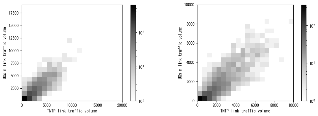
The above figures show the comparison of link traffic volume. Roughly speaking, they are mostly correlated.
[39]:
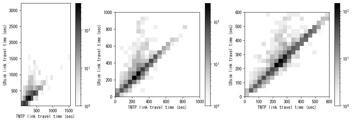
print("all links")
figure(figsize=(12,4))
subplot(131, aspect="equal")
hist2d(res_tntp_sec, res_uxsim_sec, bins=20, cmap="Greys", norm=mpl.colors.LogNorm())
xlabel("TNTP link travel time (sec)")
ylabel("UXsim link travel time (sec)")
colorbar()

subplot(132, aspect="equal")
hist2d(res_tntp_sec, res_uxsim_sec, bins=20, range=[[0,1000], [0,1000]], cmap="Greys", norm=mpl.colors.LogNorm())
xlabel("TNTP link travel time (sec)")
ylabel("UXsim link travel time (sec)")
colorbar()

subplot(133, aspect="equal")
hist2d(res_tntp_sec, res_uxsim_sec, bins=20, range=[[0,600], [0,600]], cmap="Greys", norm=mpl.colors.LogNorm())
xlabel("TNTP link travel time (sec)")
ylabel("UXsim link travel time (sec)")
colorbar()

tight_layout()
show()


print("links with non-small traffic volume only. This is because travel time of links with small traffic volume is almost equal to free flow travel time and may not be meaningful comparison")
threth = 2000
figure(figsize=(12,4))
subplot(131, aspect="equal")
hist2d(res_tntp_sec[res_tntp_vol>threth], res_uxsim_sec[res_tntp_vol>threth], bins=20, cmap="Greys", norm=mpl.colors.LogNorm())
xlabel("TNTP link travel time (sec)")
ylabel("UXsim link travel time (sec)")
colorbar()

subplot(132, aspect="equal")
hist2d(res_tntp_sec[res_tntp_vol>threth], res_uxsim_sec[res_tntp_vol>threth], bins=20, range=[[0,1000], [0,1000]], cmap="Greys", norm=mpl.colors.LogNorm())
xlabel("TNTP link travel time (sec)")
ylabel("UXsim link travel time (sec)")
colorbar()

subplot(133, aspect="equal")
hist2d(res_tntp_sec[res_tntp_vol>threth], res_uxsim_sec[res_tntp_vol>threth], bins=20, range=[[0,600], [0,600]], cmap="Greys", norm=mpl.colors.LogNorm())
xlabel("TNTP link travel time (sec)")
ylabel("UXsim link travel time (sec)")
colorbar()

tight_layout()
show()
all links
links with non-small traffic volume only. This is because travel time of links with small traffic volume is almost equal to free flow travel time and may not be meaningful comparison
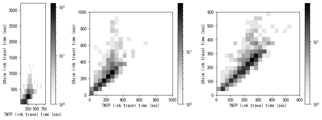
The above figures show the comparison of link traffic travel time. You can see a clear 45-degree line, suggesting that both results are similar for many links.
However, there is a noticeable difference that many links in UXsim experienced substantially longer travel time than TNTP. This is a reasonable result, because in dynamic traffic assignment with hard traffic capacity, traffic congestion can grow significantly and extend to the upstream links if the demand exceeds the capacity. This kind of realistic phenomena is not captured by the static traffic assignment model.
Now we compare the total travel time in the entire network. As shown in below, the results are not so different. From these results, we can say that UXsim output a plausible result for this scenario.
[40]:
print("total travel time (h)")
print("TNTP:\t", sum(res_tntp_sec*res_tntp_vol)/3600)
print("UXsim:\t", sum(res_uxsim_sec*res_uxsim_vol)/3600)
total travel time (h)
TNTP:    311681.3229930834
UXsim:   347367.7123302059
Code to translate TNTP files to UXsim scenario
Below is the code used to generate chicago_sketch.uxsim_scenario from TNTP datasets. To execute this code, please obtain TNTP files from TNTP repo and place them to appropriate path in advance. This code is applicable to other TNTP files with slight modifications.
[ ]:
import numpy as np
import pandas as pd
from tqdm.notebook import tqdm

from uxsim import *

############################################
# tntp parser customized for Chicago-sketch
############################################

def import_links(filename):
    """
    Modified from `parsing networks in Python.ipynb` in https://github.com/bstabler/TransportationNetworks
    Credit: Transportation Networks for Research Core Team. Transportation Networks for Research. https://github.com/bstabler/TransportationNetworks. Accessed 2021-10-01.
    """
    net = pd.read_csv(filename, skiprows=8, sep='\t')

    trimmed= [s.strip().lower() for s in net.columns]
    net.columns = trimmed

    # And drop the silly first andlast columns
    net.drop(['~', ';'], axis=1, inplace=True)
    return net

def import_nodes(filename):
    """
    Modified from `parsing networks in Python.ipynb` in https://github.com/bstabler/TransportationNetworks
    Credit: Transportation Networks for Research Core Team. Transportation Networks for Research. https://github.com/bstabler/TransportationNetworks. Accessed 2021-10-01.
    """
    net = pd.read_csv(filename, skiprows=0, sep='\t')

    trimmed= [s.strip().lower() for s in net.columns]
    net.columns = trimmed

    net.drop([';'], axis=1, inplace=True)

    return net

def import_odmatrix_chicago(matfile, nodefile):
    """
    Modified from `parsing networks in Python.ipynb` in https://github.com/bstabler/TransportationNetworks
    Credit: Transportation Networks for Research Core Team. Transportation Networks for Research. https://github.com/bstabler/TransportationNetworks. Accessed 2021-10-01.
    """
    f = open(matfile, 'r')
    all_rows = f.read()
    blocks = all_rows.split('Origin')[1:]
    matrix = {}
    for k in range(len(blocks)):
        orig = blocks[k].split('\n')
        dests = orig[1:]
        orig=int(orig[0])

        d = [eval('{'+a.replace(';',',').replace(' ','') +'}') for a in dests]
        destinations = {}
        for i in d:
            destinations = {**destinations, **i}
        matrix[orig] = destinations
    zones = max(matrix.keys())

    # mat = np.zeros((zones, zones))
    # for i in range(zones):
    #     for j in range(zones):
    #         # We map values to a index i-1, as Numpy is base 0
    #         mat[i, j] = matrix.get(i+1,{}).get(j+1,0)

    mat = [[0 for i in range(zones)] for j in range(zones)]
    for i in range(zones):
        for j in range(zones):
            # We map values to a index i-1, as Python is base 0
            mat[i][j] = matrix.get(i+1,{}).get(j+1,0)

    index = np.arange(zones) + 1

    nodelist = [i for i in range(387)]#list(import_nodes(nodefile)["node"])

    df = pd.DataFrame(mat, columns=nodelist)
    df["origin"] = nodelist
    df = df.reindex(columns=["origin"]+nodelist)
    return df

df_nodes = import_nodes("_private_files/ChicagoSketch_node.tntp")
df_links = import_links("_private_files/ChicagoSketch_net.tntp")
df_demand = import_odmatrix_chicago("_private_files/ChicagoSketch_trips.tntp", "_private_files/ChicagoSketch_node.tntp")

############################################
# prepare for deleting dummy links/nodes
############################################

map_dummy2real = {}
map_real2dummy = {}
for i in lange(df_links):
    if df_links["capacity"][i] == 49500:    #dummy link between dummy node and real node
        if df_links["init_node"][i] not in map_dummy2real.keys() and df_links["init_node"][i] < df_links["term_node"][i]:
            #print("delete: link", (df_links["init_node"][i], df_links["term_node"][i]), end=", ")
            map_dummy2real[df_links["init_node"][i]] = df_links["term_node"][i]
print("")

############################################
# uxsim setup
############################################


W = World(
    name="",
    deltan=30,
    tmax=10000,
    print_mode=1, save_mode=1, show_mode=1,
    random_seed=42,
    vehicle_logging_timestep_interval=1,
    meta_data = {"DATA SOURCE AND LICENCE": "Chicago-Sketch network. This is based on https://github.com/bstabler/TransportationNetworks/tree/master/Chicago-Sketch by Transportation Networks for Research Core Team. Users need to follow their licence. Especially, this data is for academic research purposes only, and users must indicate the source of any dataset they are using in any publication that relies on any of the datasets provided in this web site."}
)

for i in range(len(df_nodes)):
    if i+1 not in map_dummy2real.keys():
        name = str(i+1)
        x = float(df_nodes["x"][i])
        y = float(df_nodes["y"][i])
        W.addNode(name, x, y)

for i in range(len(df_links)):
    start_node = df_links["init_node"][i]
    end_node = df_links["term_node"][i]

    if start_node in map_dummy2real.keys() or end_node in map_dummy2real.keys():    #delete dummy node
        continue

    length = df_links["length"][i]*1609.34  #mile to m
    if length < 100:
        length = 100

    capacity = df_links["capacity"][i]/3600
    n_lanes = int(capacity/0.5) #based on the assumption that flow capacity per lane is 0.5 veh/s in arterial roads
    if n_lanes < 1:
        n_lanes = 1
    if df_links["link_type"][i] == 2:   #highway
        n_lanes = 3

    free_flow_time = df_links["free_flow_time"][i]*60
    if free_flow_time > 0:
        free_flow_speed = length/free_flow_time
    else:
        free_flow_speed = 10
    if free_flow_speed < 10:
        free_flow_speed = 10
    elif free_flow_speed > 40:
        free_flow_speed = 40

    W.addLink(str(i), str(start_node), str(end_node), length=length, free_flow_speed=free_flow_speed, number_of_lanes=n_lanes)


demand_multipiler = 1/0.85  #compensete some demands that are filtered out by pre-processing
demand_threthhold = 30  #delete too small demand (<= deltan) as they cause peculiar traffic pattern at the beginning of simulation
for i in tqdm(range(len(df_demand))):
    origin = str(i+1)
    if int(origin) in map_dummy2real.keys():
        origin = str(map_dummy2real[int(origin)])
    for j in range(len(df_demand)):
        destination = str(j+1)

        if int(destination) in map_dummy2real.keys():
            destination = str(map_dummy2real[int(destination)])

        if origin == destination:
            continue

        demand = df_demand.loc[i, j]*demand_multipiler
        if demand > demand_threthhold:
            try:
                W.adddemand(origin, destination, 0, 3600, volume=demand)
            except:
                print("inconsistent demand:", origin, destination, demand)

W.save_scenario("out/chicago_sketch.uxsim_scenario")

W.exec_simulation()
W.analyzer.print_simple_stats()

W.analyzer.network_fancy(animation_speed_inverse=15, sample_ratio=0.2, interval=5, trace_length=10,  figsize=6, antialiasing=False)