Network data import from OpenStreetMap
This notebook demonstrates how to import network data from OpenStreetMap (OSM). This is enabled by OSMnx (github), a Python package for OSM data handling. OSMnx is an optional module for UXsim. If you haven’t installed it, please install it first.
WARNING: Import from OSM is experimental and may not work as expected. It is functional but may produce inappropriate networks for simulation, such as too many nodes, too many deadends, fragmented networks.
Network import
Now, define UXsim World as always.
[1]:
%matplotlib inline
%load_ext autoreload
%autoreload 2
[2]:
from uxsim import *
from uxsim.OSMImporter import OSMImporter

W = World(
    name="",
    deltan=5,
    tmax=7200,
    print_mode=1, save_mode=1, show_mode=0,
    random_seed=0
)
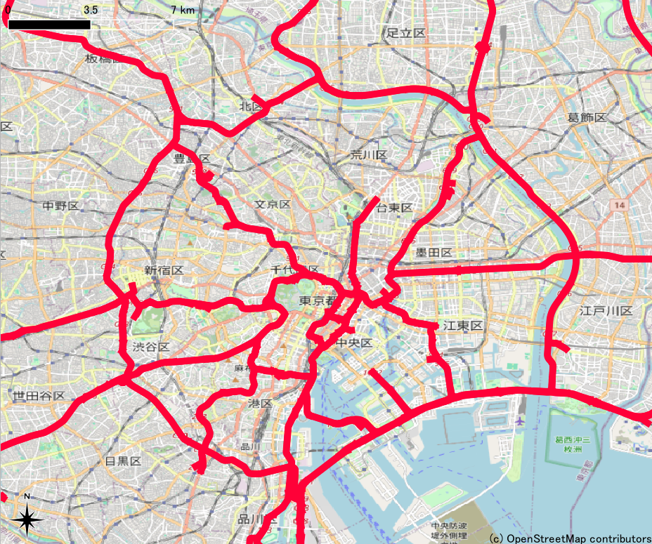
We are going to import the highway network in Tokyo. The map of the network is shown below.
[3]:
from IPython.display import display, Image
with open("dat/osm_tokyo.png", "rb") as f:
    display(Image(data=f.read(), format='png'))
OSMImporter class summarizes the import and related functions.
The area is specified by lon/lat coordinates.
custom_filter='["highway"~"motorway"]' means only motorway links are imported. If you want to import major arterial roads, you may use custom_filter='["highway"~"trunk|primary"]'. For the details, please see OSMnx documentation.
[4]:
nodes, links = OSMImporter.import_osm_data(bbox=(139.583, 35.570, 139.881, 35.817), custom_filter='["highway"~"motorway"]')
WARNING: Import from OSM is experimental and may not work as expected. It is functional but produces inappropriate networks for simulation, such as too many nodes, too many deadends, fragmented networks.
UserWarning: Import from OSM is experimental and may not work as expected. It is functional but produces inappropriate networks for simulation, such as too many nodes, too many deadends, fragmented networks.
Start downloading OSM data. This may take some time.
Download completed
imported network size:
 number of links: 812
 number of nodes: 718
Below shows the imported network data.
[5]:
OSMImporter.osm_network_visualize(nodes, links, show_link_name=0)
OSMImporter.osm_network_visualize(nodes, links, show_link_name=0, xlim=[139.75, 139.76], ylim=[35.60, 35.615], figsize=(6,6))
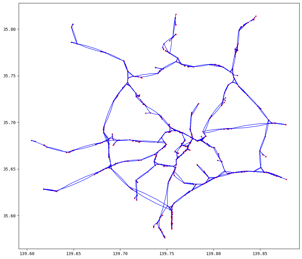
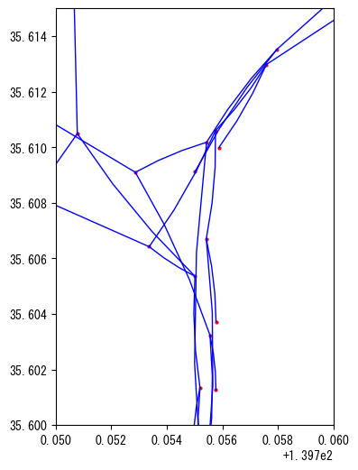
Unfortunately, the raw data is too detailed and not suitable for UXsim simulation. For example, many intersections of OSM consists of 4 nodes and may create strange traffic simulation results such as gridlocks.
Therefore, postprocessing is required to make the network suitable for simulation as follows. First, it aggregates the network by merging nodes that are closer than the threshold (0.05 degree ~= 500 m). Second, we add reverse links for each link to eliminate dead-end nodes as much as possible. Without it, a lot of vehicles will lost their way and loiter the network randomly. Please be aware that in this postprocessing the original network topology is not preserved rigorously. This function is just for convenience; if you need rigorous network data, you have to manually adjust it.
OSMImporter.osm_network_to_World will load the postprocessed network into the World.
[6]:
nodes, links = OSMImporter.osm_network_postprocessing(nodes, links, node_merge_threshold=0.005, node_merge_iteration=5, enforce_bidirectional=True)
OSMImporter.osm_network_to_World(W, nodes, links, default_jam_density=0.2, coef_degree_to_meter=111000)
aggregated network size:
 number of links: 664
 number of nodes: 274
[7]:
OSMImporter.osm_network_visualize(nodes, links, show_link_name=0)
OSMImporter.osm_network_visualize(nodes, links, show_link_name=0, xlim=[139.75, 139.76], ylim=[35.60, 35.615], figsize=(6,6))
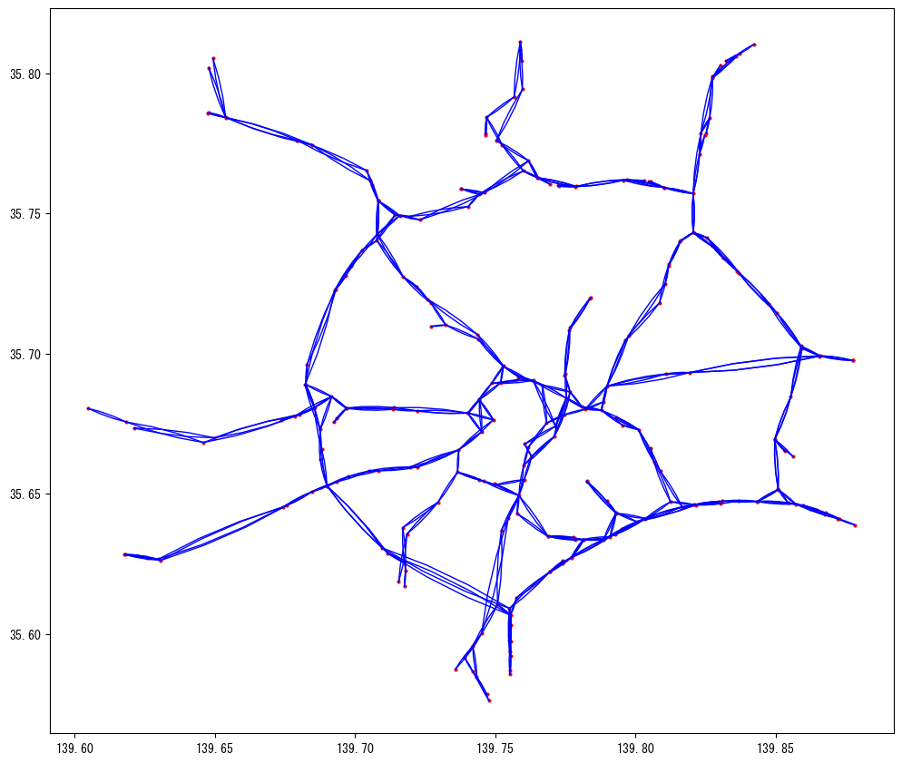
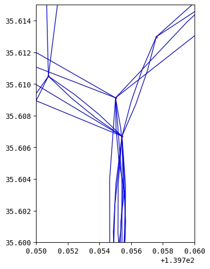
As a result, the network data is significantly simplified. For example, the highway junction is represented by fewer number of nodes which is convenient. You can see that this is still similar to the real network shown before.
Demand
The travel demand is now defined using coordinates. Below add demand from a circular area to another circular area. It represents demand to central Tokyo from surroundings.
[8]:
W.adddemand_area2area(139.70, 35.60, 0, 139.75, 35.68, 0.05, 0, 3600, volume=5000)
W.adddemand_area2area(139.65, 35.70, 0, 139.75, 35.68, 0.05, 0, 3600, volume=5000)
W.adddemand_area2area(139.75, 35.75, 0, 139.75, 35.68, 0.05, 0, 3600, volume=5000)
W.adddemand_area2area(139.85, 35.70, 0, 139.75, 35.68, 0.05, 0, 3600, volume=5000)
Simulation and results
Now you can execute the simulation.
[9]:
W.exec_simulation()
simulation setting:
 scenario name:
 simulation duration:    7200 s
 number of vehicles:     19200 veh
 total road length:      915107.2510858708 m
 time discret. width:    5 s
 platoon size:           5 veh
 number of timesteps:    1440
 number of platoons:     3840
 number of links:        664
 number of nodes:        274
 setup time:             47.44 s
simulating...
      time| # of vehicles| ave speed| computation time
       0 s|        0 vehs|   0.0 m/s|     0.00 s
     600 s|     2255 vehs|  12.8 m/s|     2.09 s
    1200 s|     5265 vehs|  11.7 m/s|     4.02 s
    1800 s|     7075 vehs|  11.2 m/s|     6.27 s
    2400 s|     7545 vehs|  10.9 m/s|     8.53 s
    3000 s|     7435 vehs|  10.7 m/s|    10.81 s
    3600 s|     7630 vehs|  11.0 m/s|    13.29 s
    4200 s|     5205 vehs|  10.0 m/s|    15.37 s
    4800 s|     2850 vehs|   8.0 m/s|    16.95 s
    5400 s|     1635 vehs|   7.0 m/s|    18.10 s
    6000 s|      850 vehs|   8.5 m/s|    19.10 s
    6600 s|      265 vehs|   9.7 m/s|    20.04 s
    7195 s|       25 vehs|   8.3 m/s|    20.38 s
 simulation finished
[9]:
1
[10]:
W.analyzer.print_simple_stats()
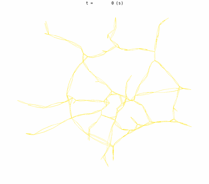
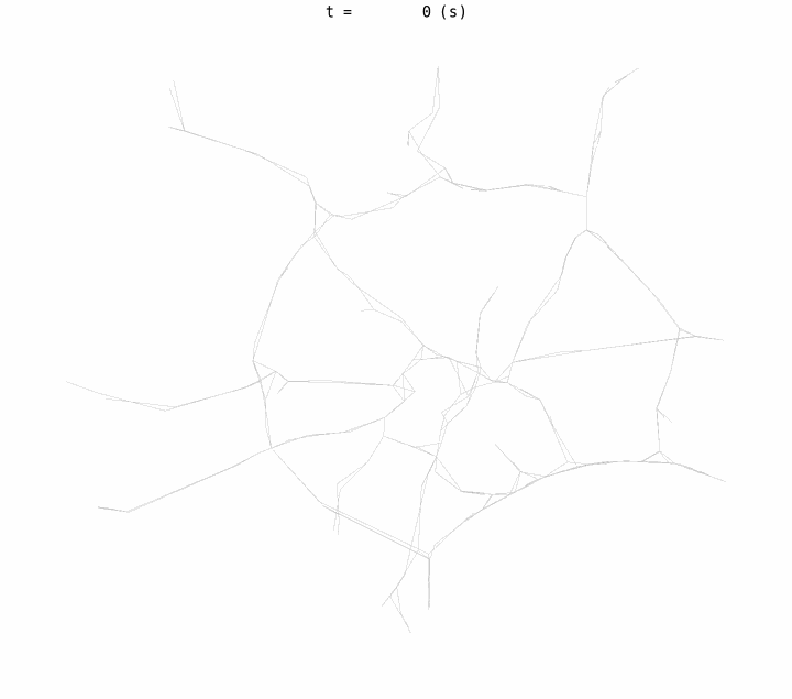
W.analyzer.network_anim(animation_speed_inverse=15, detailed=0, network_font_size=0)
W.analyzer.network_fancy(animation_speed_inverse=15, sample_ratio=0.1, interval=10, trace_length=5)
from IPython.display import display, Image
with open("out/anim_network0.gif", "rb") as f:
display(Image(data=f.read(), format='png'))
with open("out/anim_network_fancy.gif", "rb") as f:
display(Image(data=f.read(), format='png'))
results:
 average speed:  10.7 m/s
 number of completed trips:      19175 / 19200
 average travel time of trips:   1695.5 s
 average delay of trips:         428.7 s
 delay ratio:                    0.253
 generating animation...
generating animation...
Now we get somewhat plausible results. Traffic from outskirts goes to the central Tokyo, causing traffic congestion due to the concentration.
Note that the above result is not very realistic. To obtain realistic results, you have to calibrate demands and scenario parameters very carefully. This usually requires hard work.